UCL CASA The Bartlett UrbanAI 2026

Shaping
Cool Cities

Multi-source data fusion for modelling urban heat mitigation across six European cities

Gerardo Ezequiel Martin Carreno

MSc Urban Spatial Science · UCL

Multi-source data fusion: satellite, street network, and street-level views converging to map urban heat and cooling

Six cities · Five data sources · 118 features · Open data

WhyHowFindingsAction

61,000

Deaths from heat across Europe.
One summer. 2022.

Among the deadliest natural disasters in modern European history.
Streets designed to maximise winter sunlight had become heat traps.

Ballester et al. (2023) Nature Medicine

WhyHowFindingsAction

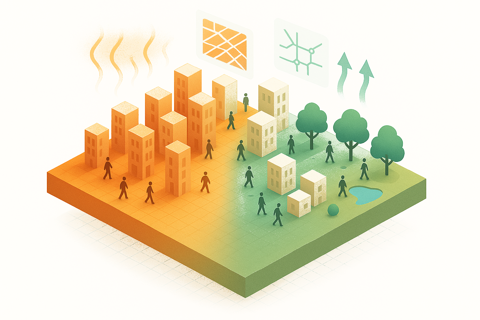
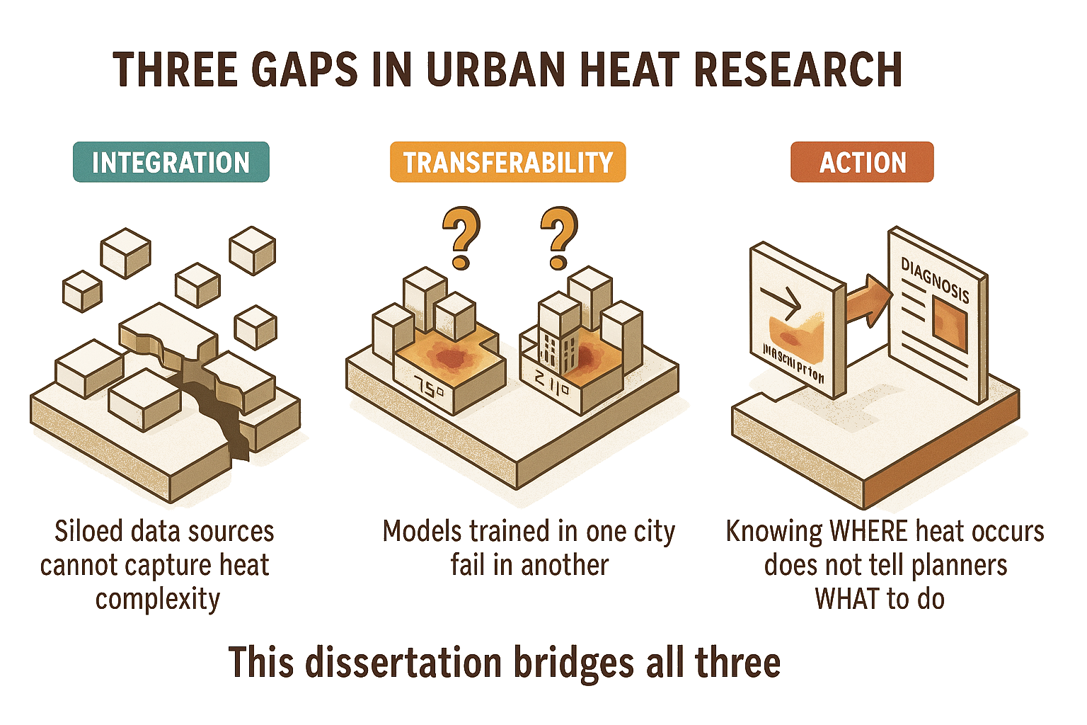
Three Gaps Preventing Action

Integration

Studies look at buildings, trees, or streets separately. Heat comes from how they interact.

Transferability

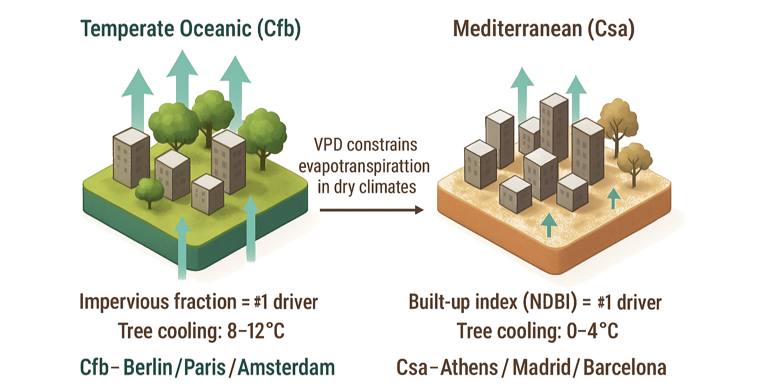
The same tree cools 8–12°C in Berlin but only 0–4°C in Athens. Same strategy, different results.

Action

Planners need the where, the why, and the how. Most models only give the first.

RQ1: What drives urban heat across contexts?

RQ2: Where should cities intervene to protect the most vulnerable?

Three research gaps: Integration, Transferability, and Action

Schwaab et al. (2021) Nat. Comms. · Camps-Valls et al. (2025) Nature Communications. · Lundberg & Lee (2017) SHAP.

WhyHowFindingsAction

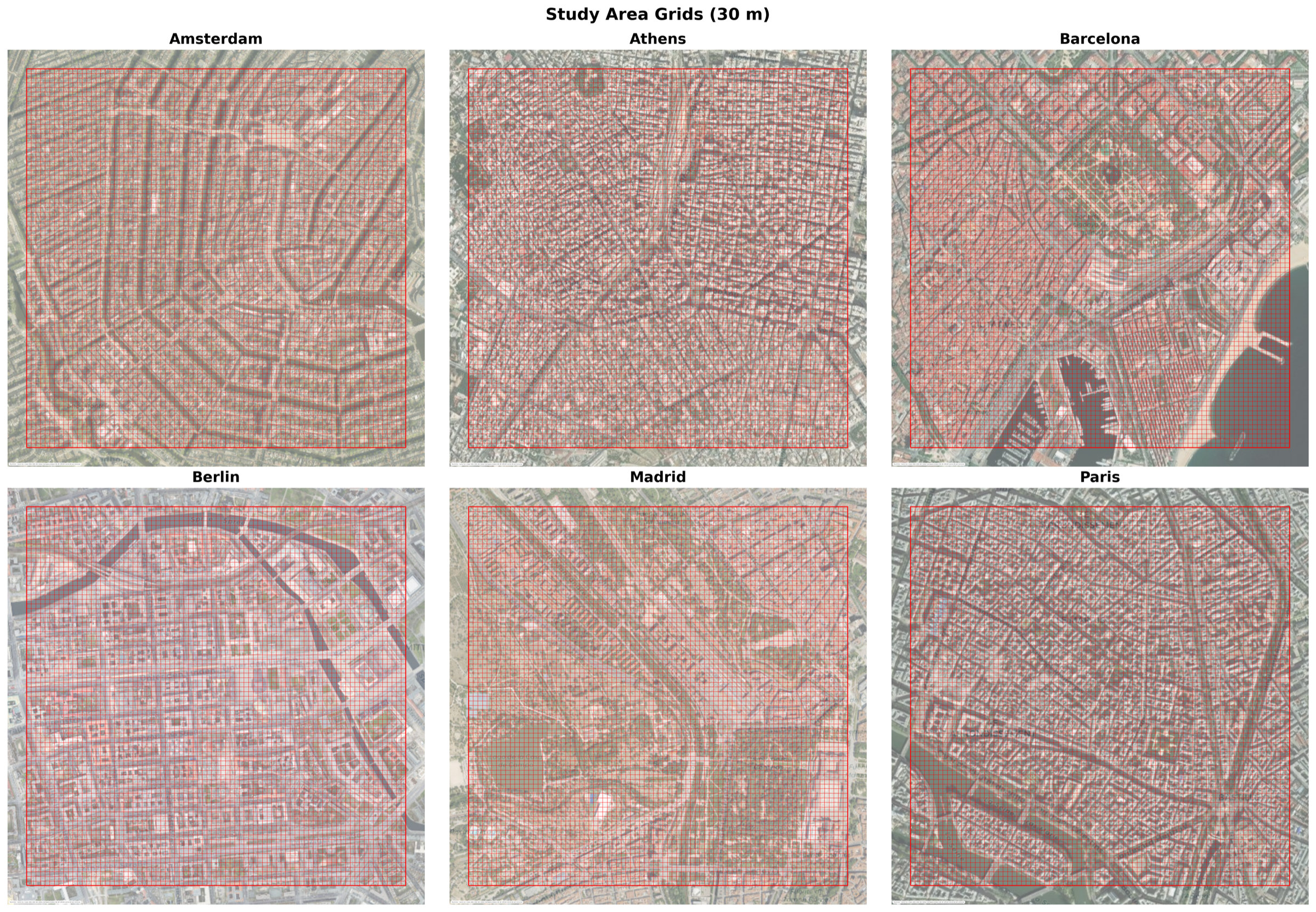
Six Cities, Three Climates

Oceanic (Cfb): Amsterdam, Paris

Mediterranean (Csa): Athens, Barcelona

Transitional: Berlin Cfb/Dfb · Madrid Csa/BSk

40,344 grid cells at 30m resolution · ~6 km² per city

30m study area grids across six European cities

Stewart & Oke (2012) BAMS. · Yap et al. (2023) Urbanity, npj Urban Sustainability.

WhyHowFindingsAction

Five Data Sources, One Framework

118 features from 5 open-source tools. Zero proprietary data. Any European city can replicate this tomorrow.

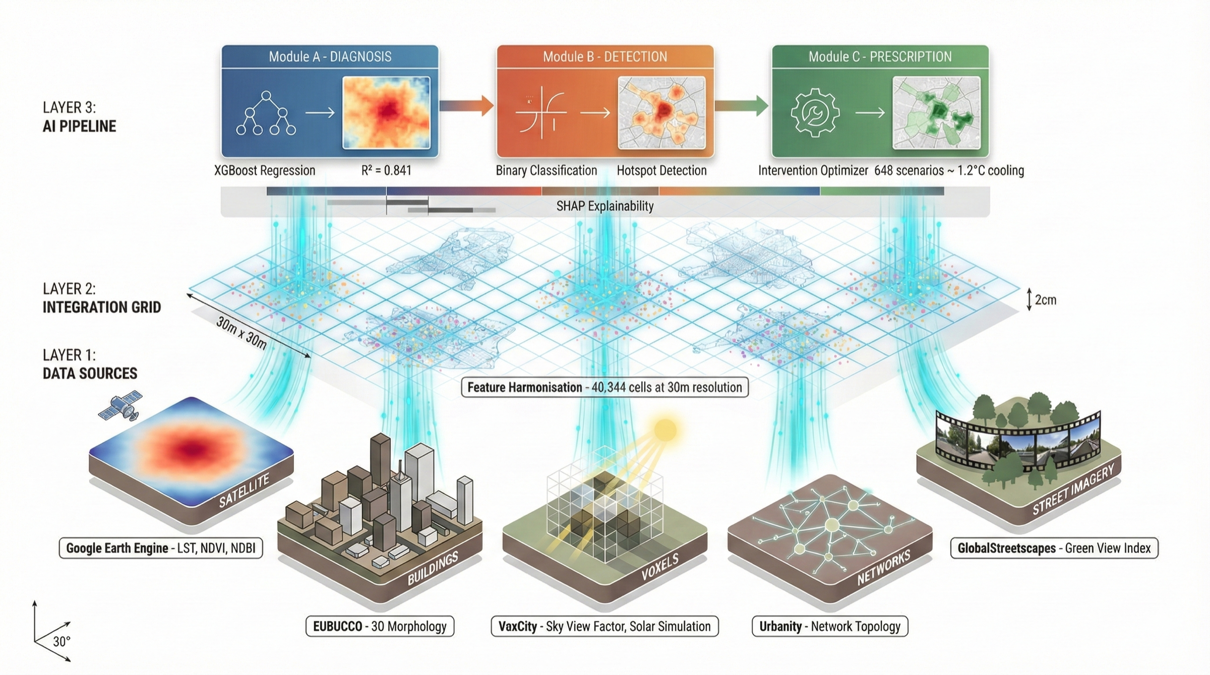
Gorelick et al. (2017) GEE · Fujiwara et al. (2026) VoxCity · Yap et al. (2023) Urbanity · Hou et al. (2024) GlobalStreetscapes · Milojevic-Dupont et al. (2023) EUBUCCO

WhyHowFindingsAction

Google Earth Engine

Landsat 30m · Surface temperature · Vegetation indices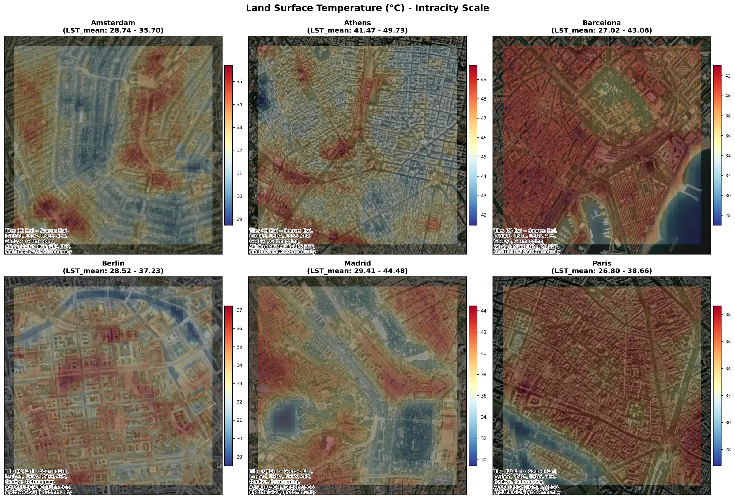

Land Surface Temperature

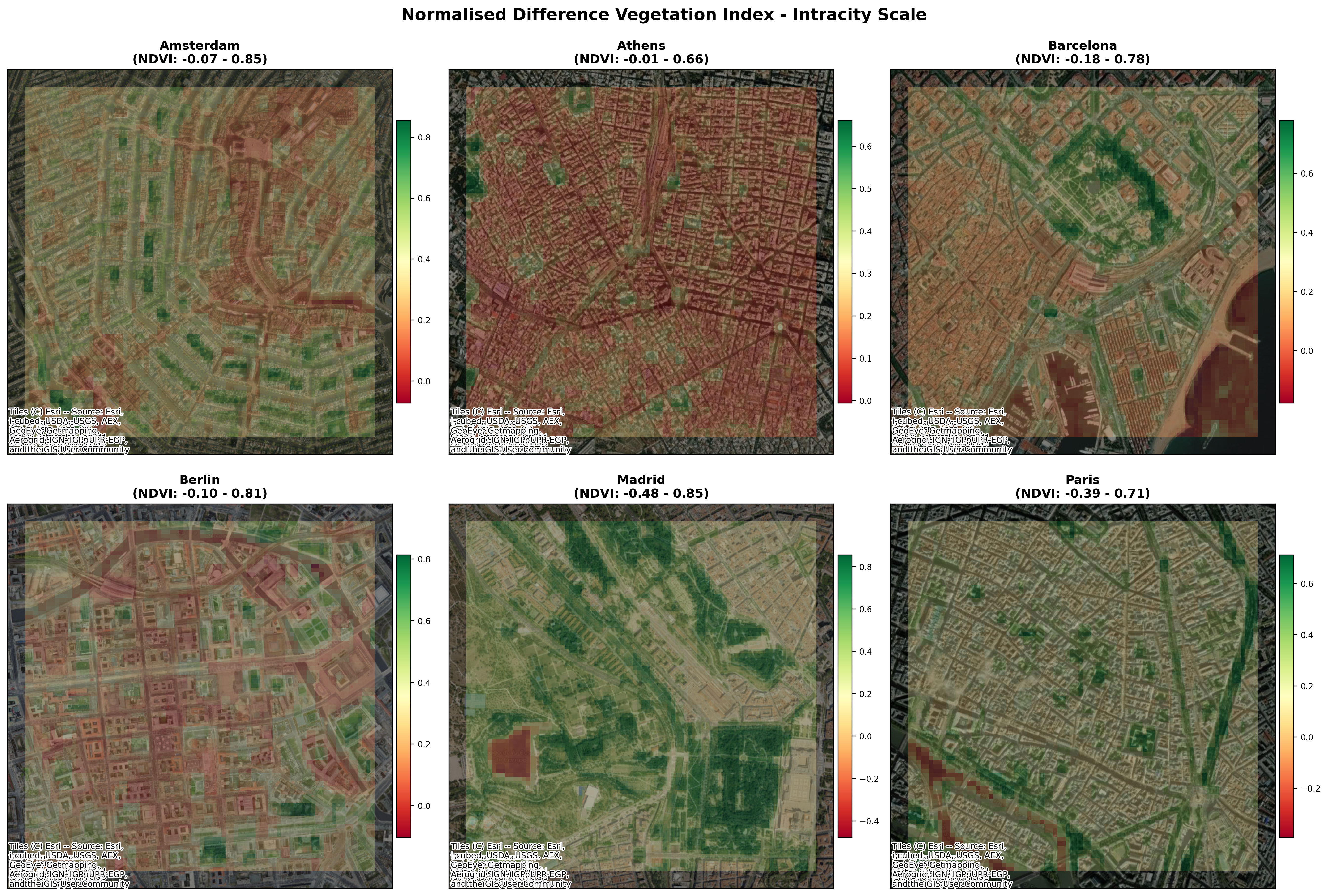NDVI Vegetation Index

Where vegetation disappears, temperatures spike. This inverse pattern is the dependent variable our model learns to predict.

Gorelick, N. et al. (2017) ‘Google Earth Engine’, Remote Sensing of Environment, 202, pp. 18-27.

WhyHowFindingsAction

Urbanity

Street network topology · Connectivity · Ventilation pathways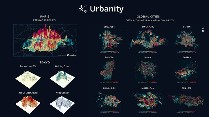

Source: Urbanity global dataset

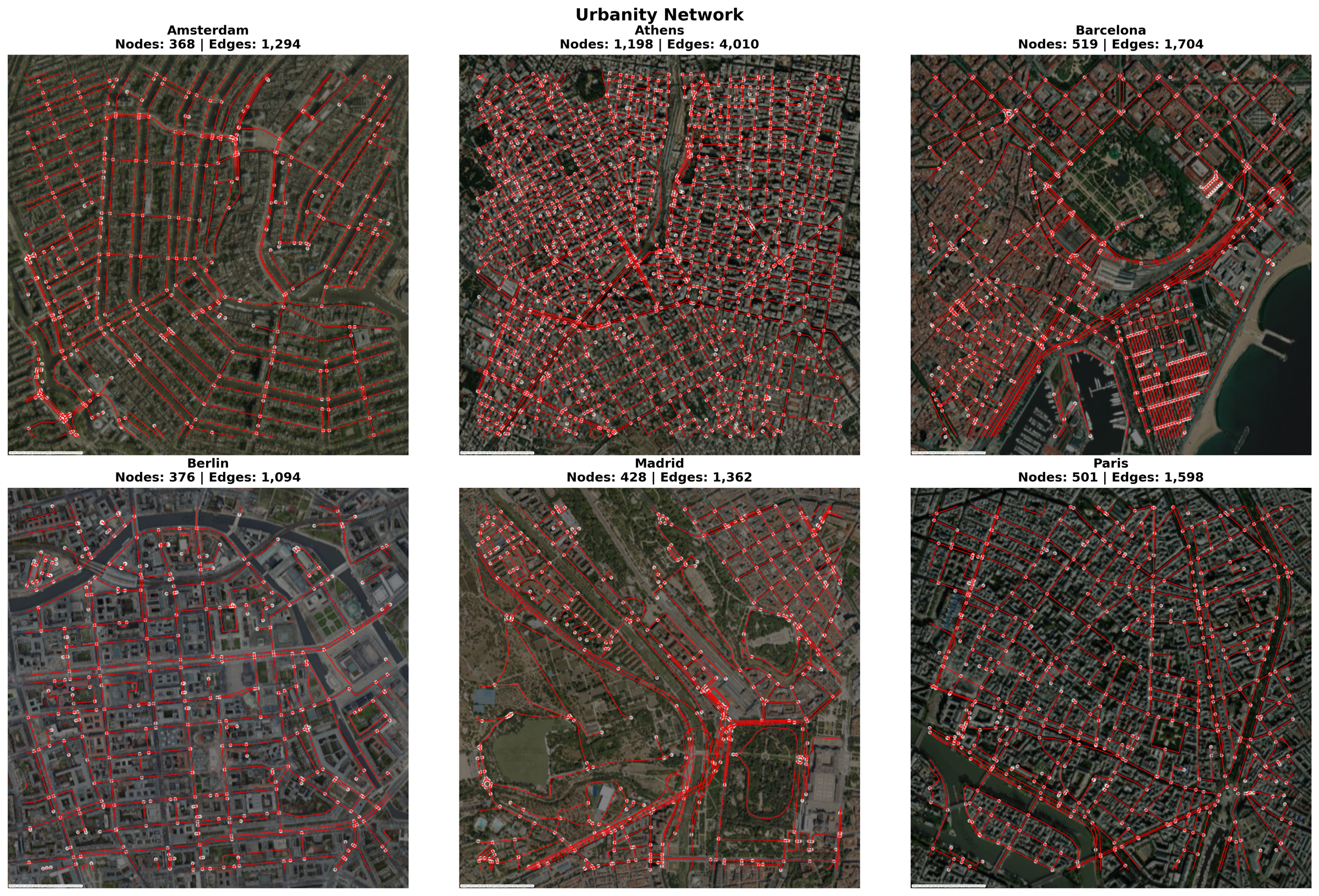Our six cities: network topology

Amsterdam’s regular canal grid channels cooling winds. Athens’s organic fabric traps them. Network topology determines whether park cooling reaches surrounding streets.

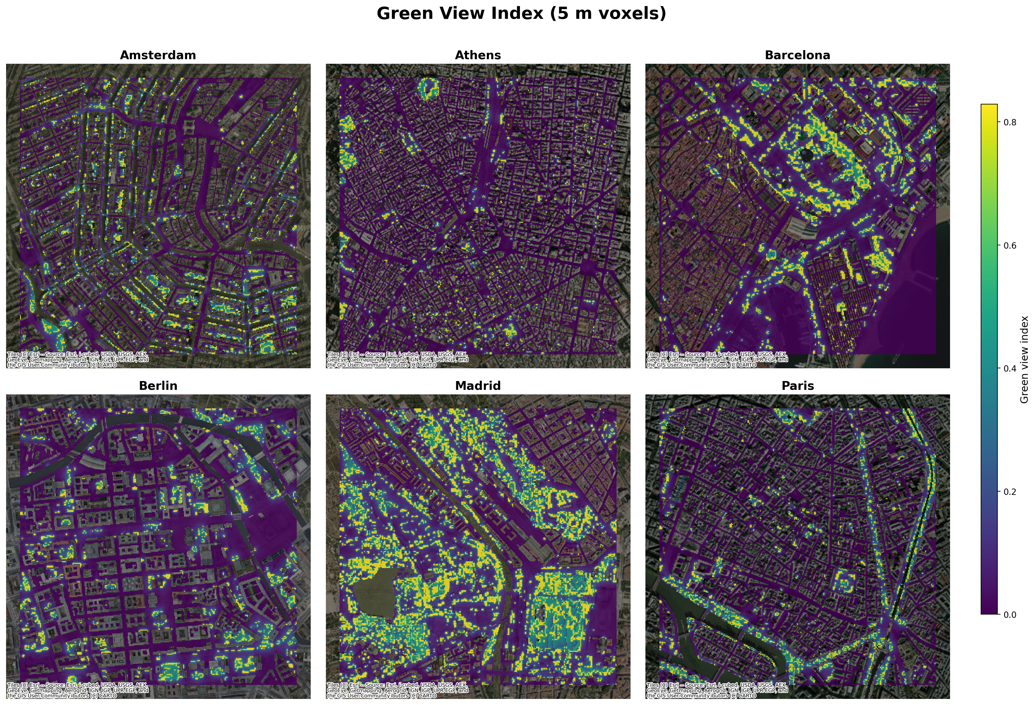
Yap, W. et al. (2023) ‘Urbanity’, npj Urban Sustainability.

WhyHowFindingsAction

GlobalStreetscapes

10 million street-level images · Green View Index · Pedestrian perspective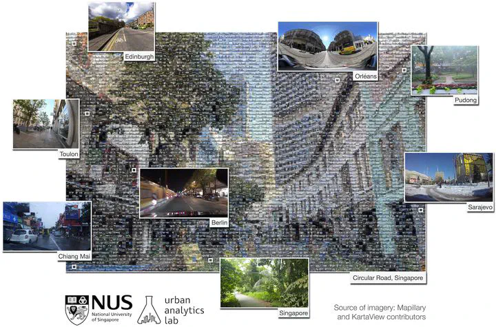

Source: 10M street-level images

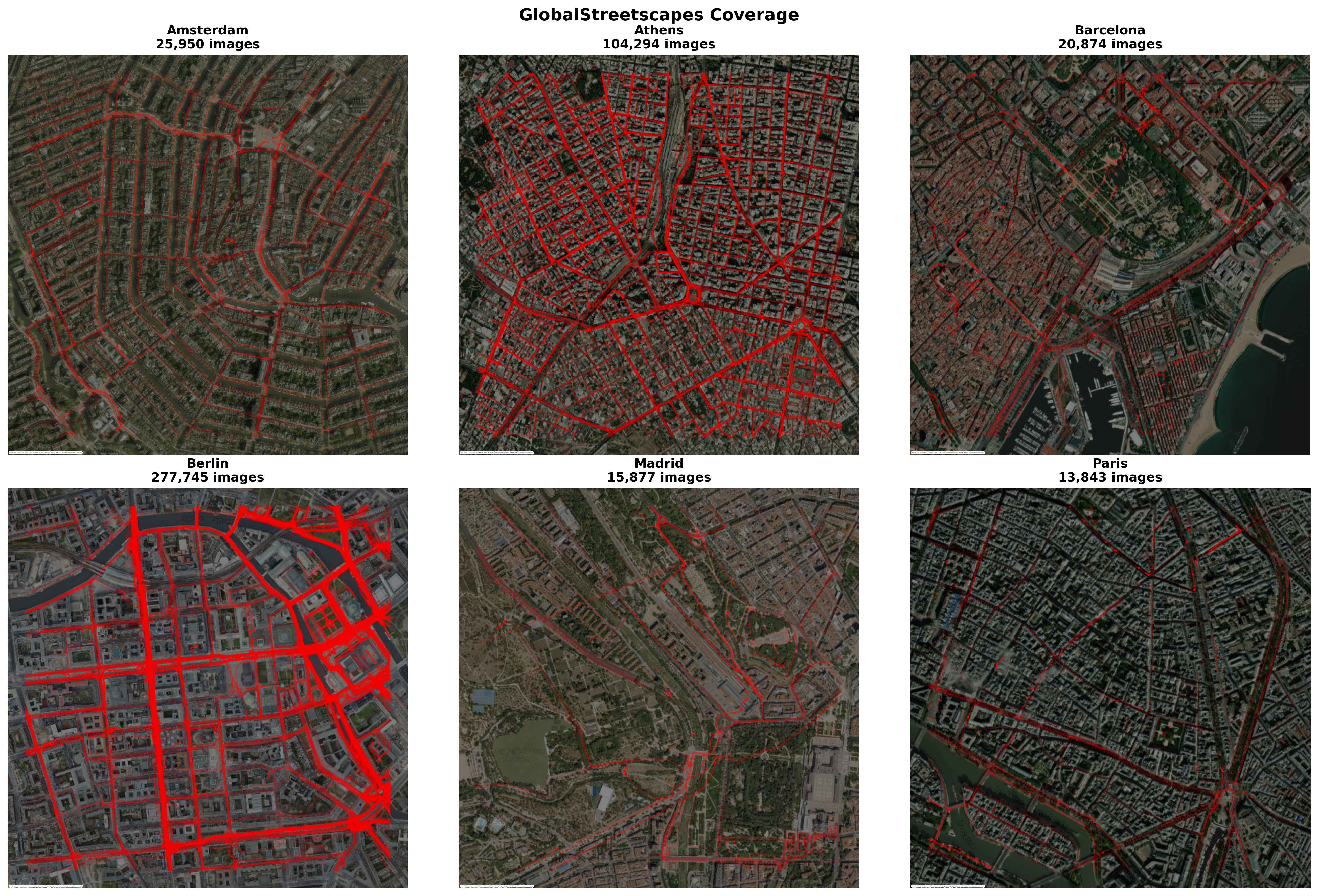Our six cities: coverage points

Satellites see canopy from above. Street imagery sees shade from below. Divergence between the two validates the multi-source approach.

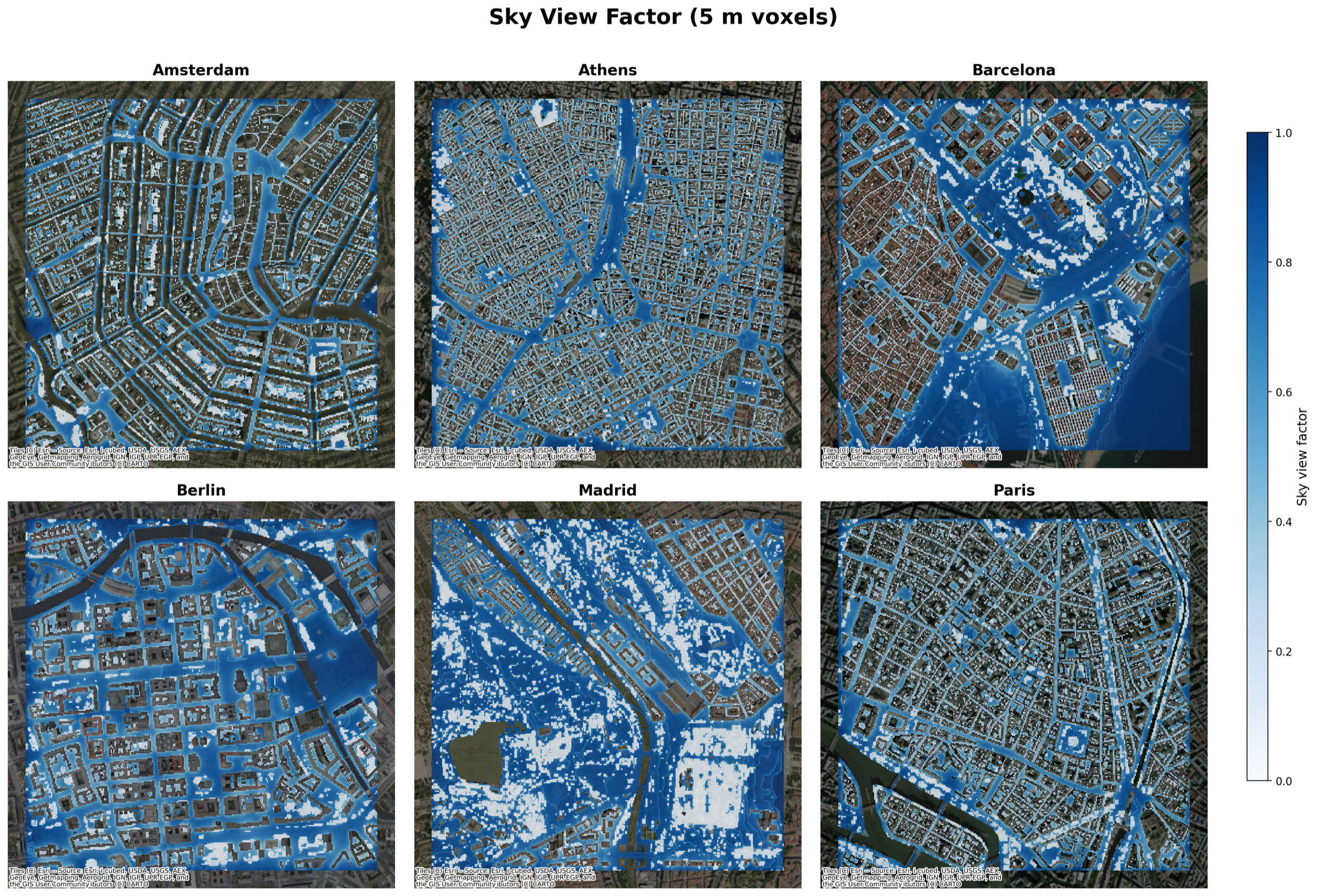
Hou, Y. et al. (2024) GlobalStreetscapes. · Li, X. et al. (2015) Green View Index.

WhyHowFindingsAction

EUBUCCO

3D building morphology · Heights · Footprints · Canyon geometry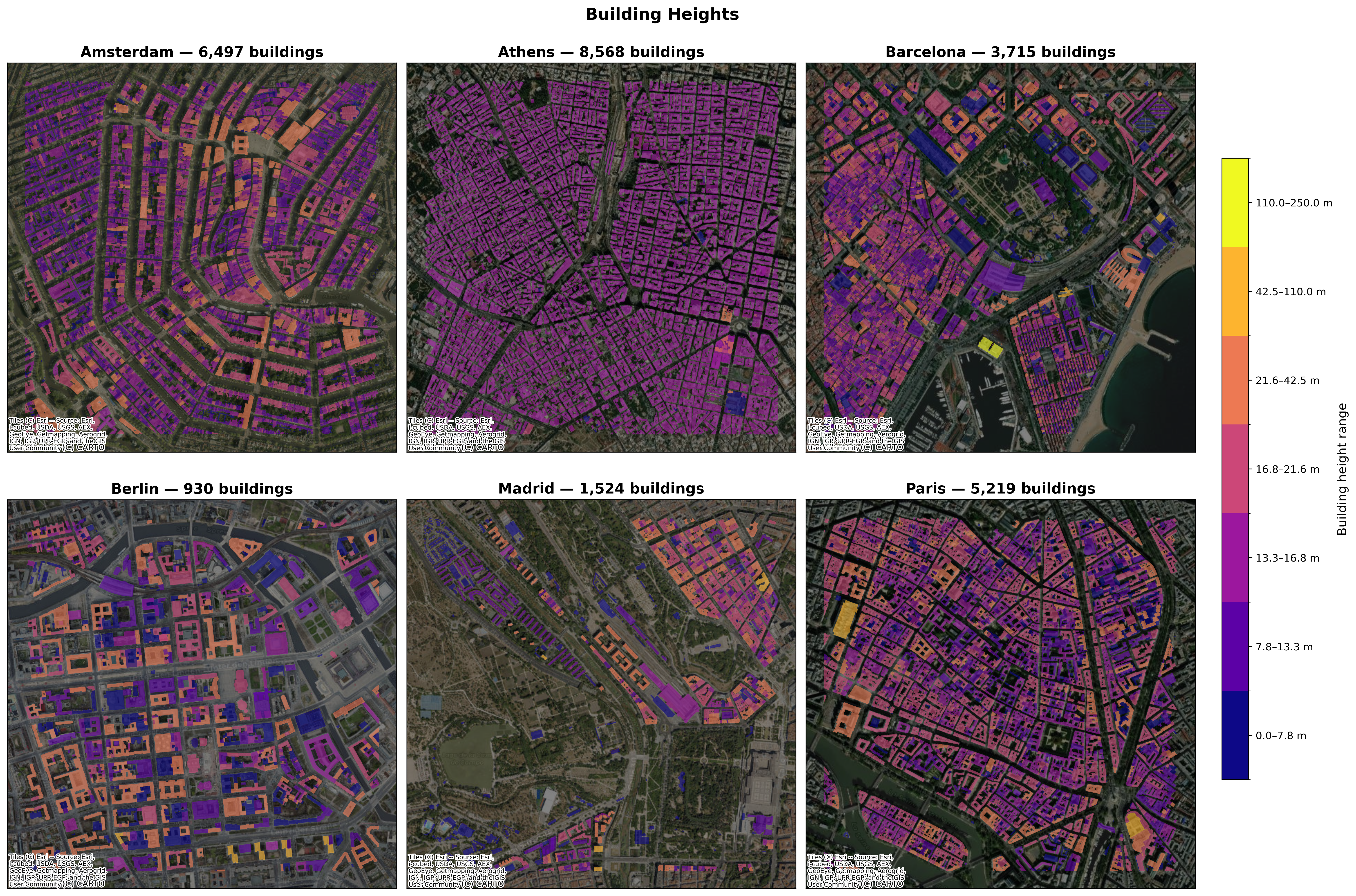

Canyon geometry drives nighttime heat retention. Paris’s uniform Haussmann fabric vs Athens’s irregular growth produce fundamentally different thermal dynamics.

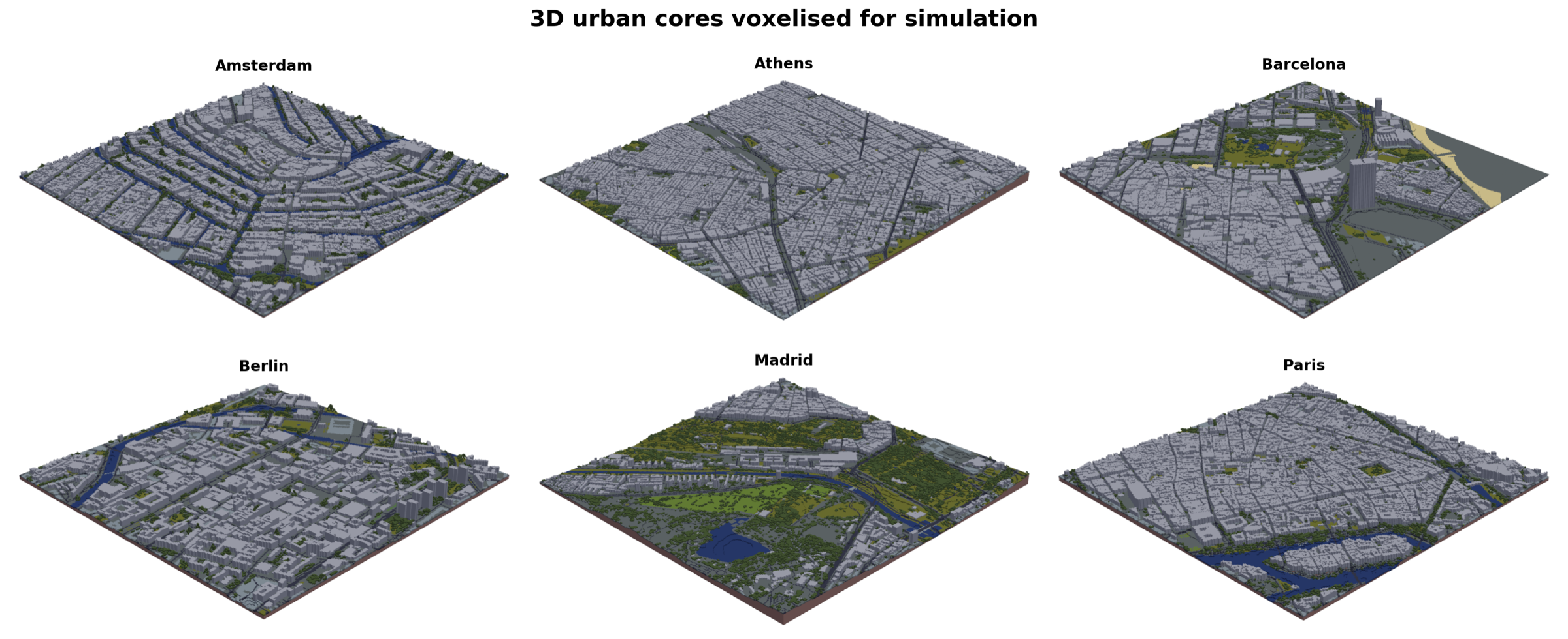
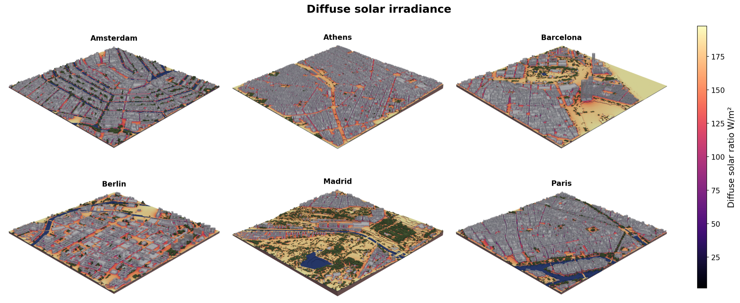
Milojevic-Dupont, N. et al. (2023) ‘EUBUCCO v0.1’, Scientific Data, 10, 146.

WhyHowFindingsAction

Six Cities in 3D

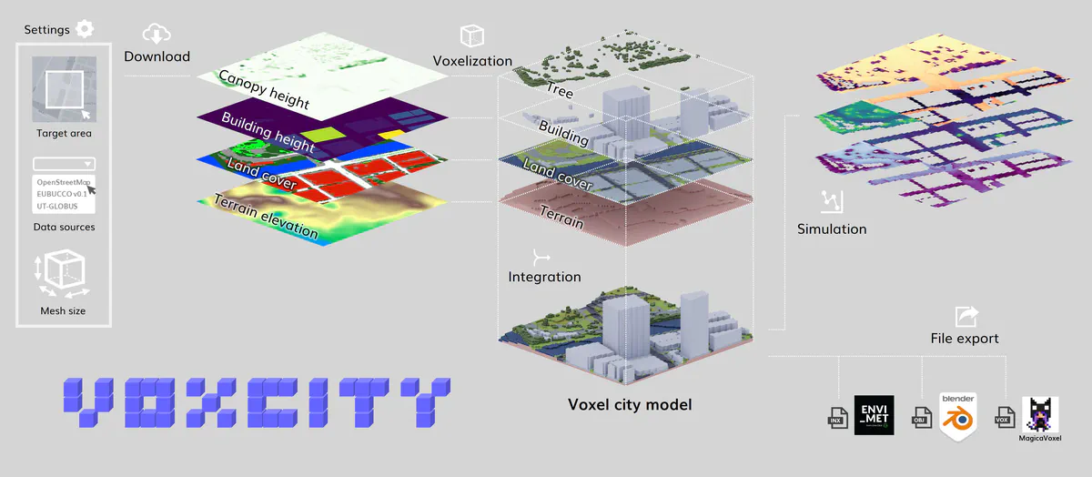VoxCity 3D city model vertical cross-section

VoxCity 3D model

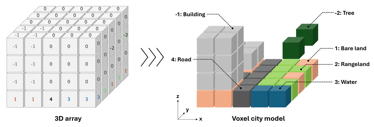3D voxel representation of urban morphology

Voxelised urban form

Diffuse solar irradiance across 6 cities

Fujiwara, K. et al. (2026) ‘VoxCity’, Computers, Environment and Urban Systems, 123, 102366. · Biljecki et al. (2015) ISPRS Int. J. Geo-Inf. · Li, X. et al. (2015) Green View Index.

[3:30 — 30s. Has 3 transitions. If behind, show geometry + GVI/SVF only.] VoxCity converts open data into 3D models at 5-metre voxel resolution. [CLICK] Six cities voxelised — dramatically different morphologies. [CLICK] Green View Index and Sky View Factor side by side. GVI: canopy from a pedestrian's perspective. SVF: how open the sky is above. Low SVF means deep canyons trapping heat at night. [CLICK] Solar irradiance — Barcelona's grid distributes heat evenly, Athens's basin traps it. Five data sources, 118 features. Now — what do we do with them? [Q&A: 5m voxels aggregated to 30m. EPW weather files, 15 June 14:00 local, TMYx 2007-2021. Ray-tracing: building shadows + canopy transmittance. SVF entered the model; solar irradiance primarily for visualisation.]

WhyHowFindingsAction

From Prediction to Prescription

XGBoost with SHAP explainability: the model shows its work at every stage. The planner keeps the final call.

Three-stage pipeline diagram: regression predicts temperature, classification identifies hotspots weighted by vulnerability, scenario grid search tests 648 intervention combinations

Chen & Guestrin (2016) XGBoost. · Lundberg & Lee (2017) SHAP. · Eyni et al. (2025) Scientific Reports.

[4:00 — 30s] Three stages. Predict temperature anomalies. Classify hotspots weighted by vulnerability. Test 648 intervention scenarios. The model shows its work — every prediction decomposes into feature contributions. The planner keeps the final call. This is augmented intelligence — AI as co-pilot, not replacement. The planner sees the receipt for every prediction and decides what to act on. [Q&A: XGBoost for exact SHAP TreeExplainer, nonlinear thresholds, mixed features. 200 Bayesian trials (Optuna). 3×9×8×3 = 648 combos, bootstrapped 500×.] [Q&A: "Why not deep learning?" — (1) Exact Shapley values vs approximate. (2) XGBoost matches/beats neural nets on tabular data (Grinsztajn 2022). (3) 40K cells modest for DL. Explainability over marginal accuracy.] [Q&A: "Not causal." — Correct. Hypotheses for field validation, not causal claims.] [Q&A: "Why not CFD?" — CFD: one block in hours. We: 40K cells across 6 cities. Complementary — our priority zones tell you WHERE to deploy CFD.] [Q&A: "New city timeline?" — Under half a day with existing Landsat. Bottleneck is vulnerability data curation.]

WhyHowFindingsAction

Regression→Classification→Scenarios

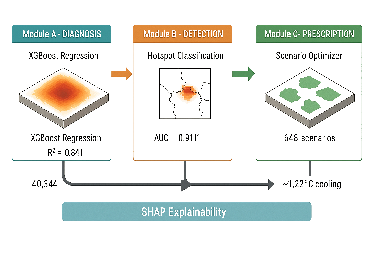
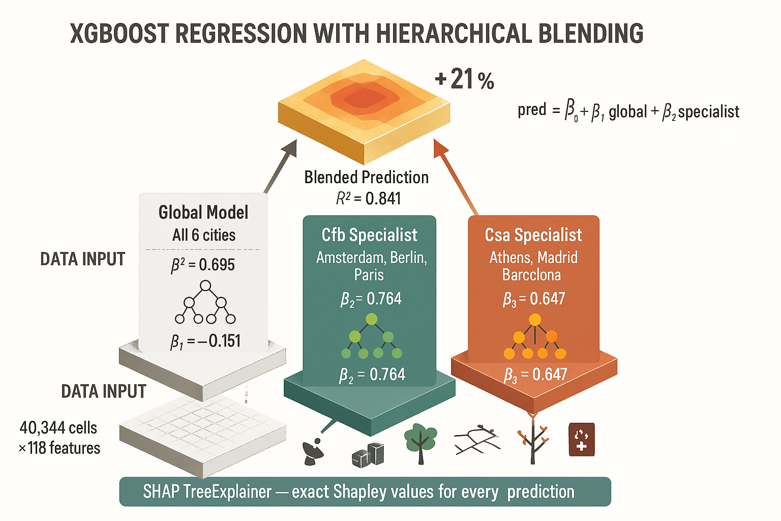
XGBoost Regression: Why This Approach?

40,344 cells · 30m resolution · 6 cities · Target: UHI anomaly (each cell’s temperature minus its city mean — not raw LST, which inflates R² to 0.97 by capturing climate, not urban form)

Why XGBoost? Heat responds non-linearly to urban form. Trees cool effectively until water stress kicks in. Sealed surfaces trap heat, but the tipping point differs by climate. We need a model that captures these thresholds and shows its reasoning.

Non-linear thresholds: captures regime changes linear models miss
SHAP explainability: every prediction decomposes into feature contributions, so the planner sees why
Hierarchical blend: global + climate-zone specialists learn what each city needs differently

Global R² 0.695 → Blended 0.841. Climate-zone specialisation cuts error by 48%.

Paris 0.93 Barcelona 0.93 Amsterdam 0.88 Athens 0.73 Berlin 0.73 Madrid 0.72

XGBoost regression with hierarchical climate-zone blending: global model (−0.151) + Cfb specialist (0.764) + Csa specialist (0.647) = blended R² 0.841

Chen & Guestrin (2016) XGBoost, KDD. · Lundberg & Lee (2017) SHAP values. · Oke et al. (2017) 300m advective transport scale.

[4:30 — 40s] Three XGBoost models — global, Mediterranean specialist, oceanic specialist — blended with learned weights. [GESTURE to diagram] The global gets subtracted — negative weight. Climate-zone specialists dominate. The blend cuts unexplained variance by 48%. Look at the city badges: Paris and Barcelona above 0.93. Athens and Berlin at 0.73. Madrid 0.72. The model works across contexts, but performance varies — and that variation is itself informative. [Q&A: Blend: pred = β₀ + β₁·global + β₂·specialist. Weights: global −0.151, Cfb 0.764, Csa 0.647. 165 features → spatial lags → 189 → correlation filter → 118. Athens blend hurts: global 0.751 → blended 0.730, basin overrides climate correction.] [Q&A GLOSSARY: R² = proportion of variation explained. SHAP = feature contribution receipt. AUC = hotspot discrimination (0.5 = coin flip, 1.0 = perfect).]

WhyHowFindingsAction

Regression→Classification→Scenarios

Can We Trust the Numbers?

Hot areas sit next to hot areas. Without careful testing, the model could just memorise where things are instead of learning why they’re hot. Five checks prevent that.

Spatial cross-validation

The model never sees its test area’s neighbours during training. 5 folds, 600m spatial blocks, stratified by heat intensity and density.

City-demeaned targets

Raw temperature R² = 0.97, but that mostly captures climate. Subtracting each city’s mean isolates what urban form does. R² = 0.84.

Scale sensitivity (MAUP)

Tested at 30m, 60m, 90m. At 60m the model loses 17% of explained variance; it falls between radiative and advective physics. 30m is the right scale.

Residual autocorrelation

Moran’s I confirms significant spatial clustering in predictions (I = 0.66–0.92, p<0.001), validating why spatial blocking was essential.

Stability & tuning

5 random seeds (σR² = 0.064). 200 Bayesian trials optimised 820 trees, depth 6, lr 0.03. Features: 165 base → 189 with spatial lags → 118 after correlation filter (|r|>0.92).

The model learns morphology, not spatial patterns.

Oke et al. (2017) Urban Climates. · Openshaw (1984) MAUP. · Anselin (1995) Moran’s I. · Roberts et al. (2017) Spatial CV. · Valavi et al. (2018) blockCV.

WhyHowFindingsAction

Regression→Classification→Scenarios

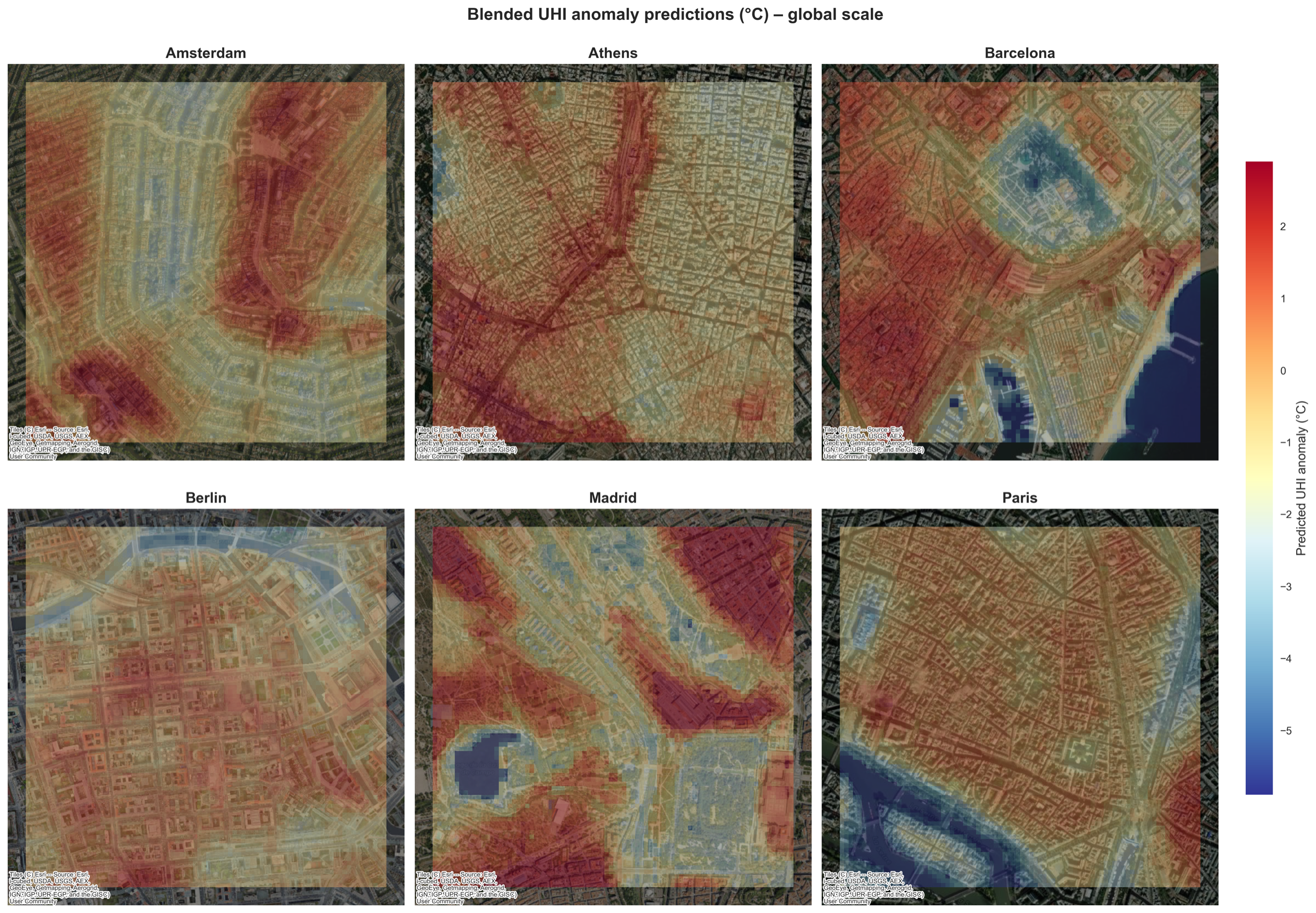
Does It Work Across Contexts?

City	R²	RMSE
Paris	0.932	0.49°C
Barcelona	0.926	0.85°C
Amsterdam	0.880	0.44°C
Athens *	0.730	0.63°C
Berlin	0.727	0.66°C
Madrid	0.718	1.53°C

The model works, but accuracy isn’t the finding. What the model reveals about what drives heat is.

* Athens R² drops with blending (−2.8%): its topographic basin overrides climate-zone correction. That’s not a failure; it’s a finding. Geography matters.

Observed vs predicted UHI spatial comparison across cities

Chen & Guestrin (2016) XGBoost, KDD. · Tanoori et al. (2024) ML for UHI benchmarks.

WhyHowFindingsAction

Regression→Classification→Scenarios

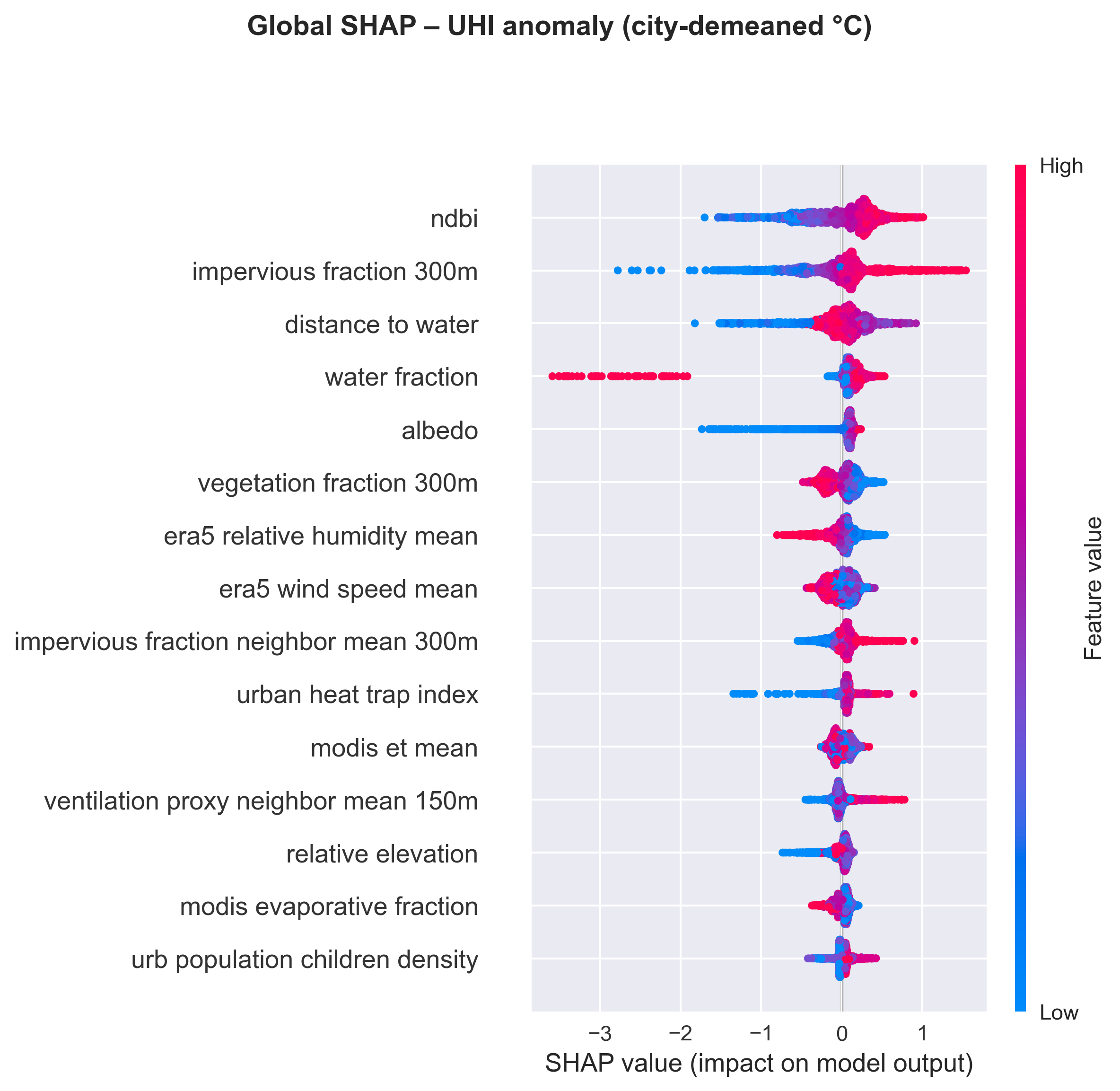
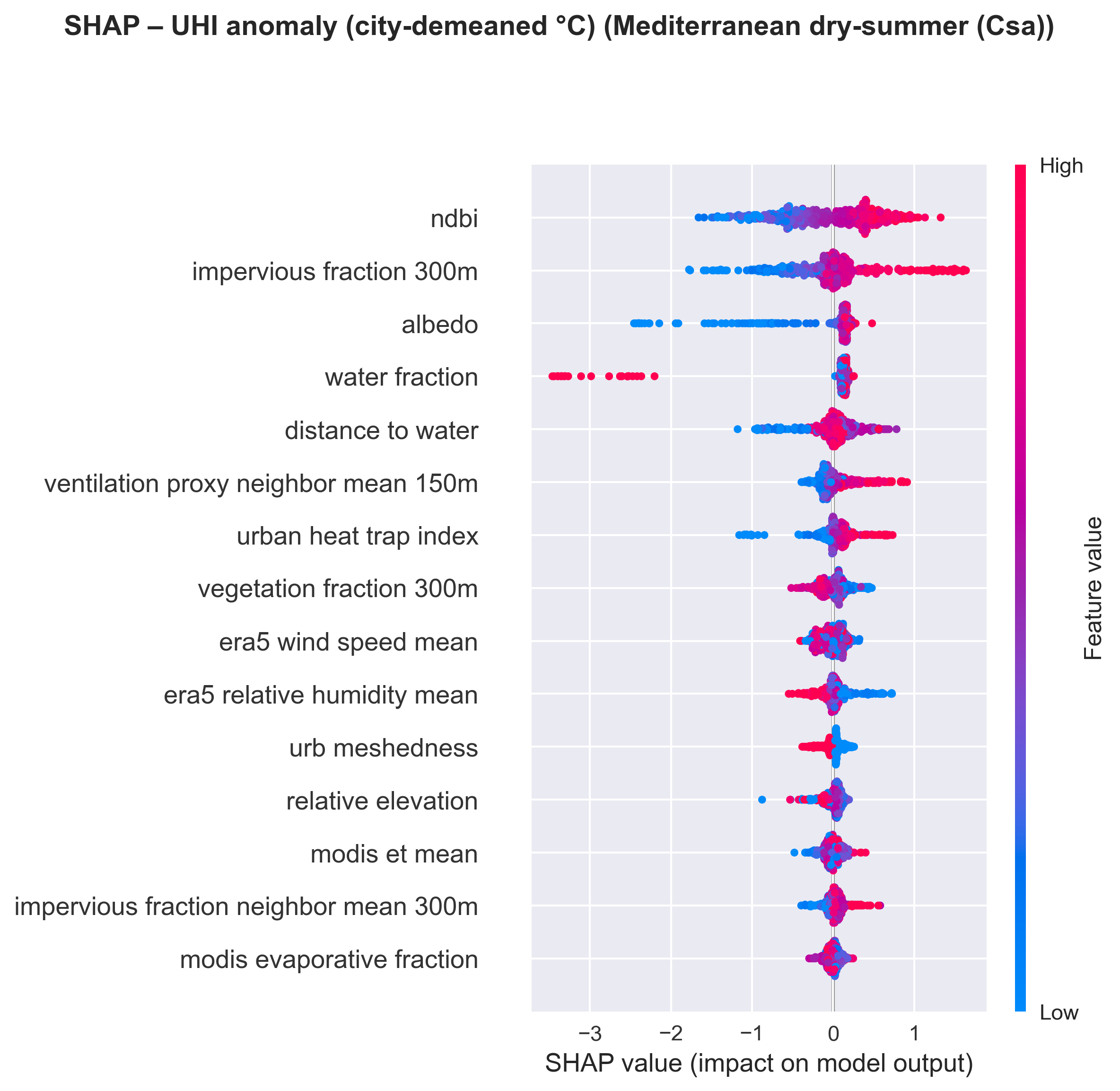
What Actually Drives Urban Heat?

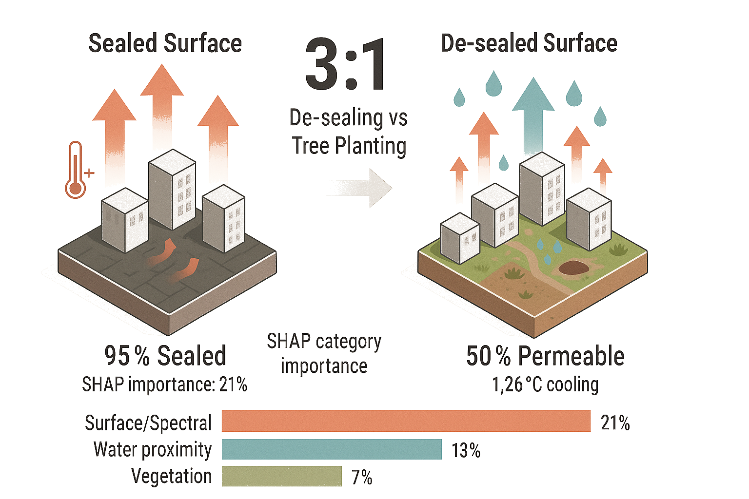
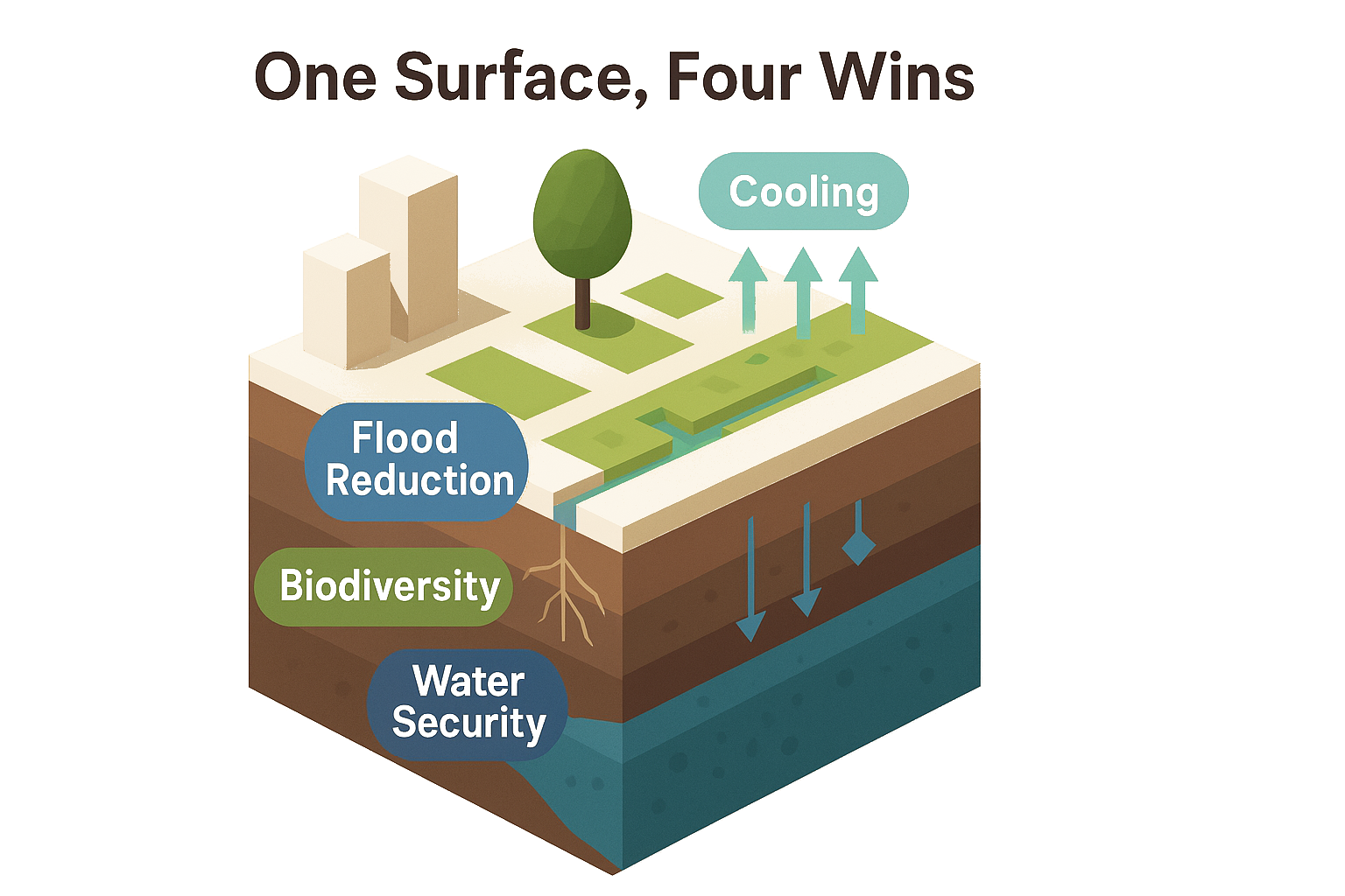
De-sealing matters 3× more than tree planting.

Trees provide shade, biodiversity, air quality. But for temperature reduction, the surface is the stronger lever.

Global SHAP feature importance beeswarm plot

Lundberg & Lee (2017) SHAP. · Schwaab et al. (2021) Nat. Comms. · Eyni et al. (2025) Scientific Reports.

[6:15 — 50s. SLOW DOWN — central finding.] SHAP decomposes every prediction into feature contributions. The hierarchy surprises: surface permeability 21%, water features 13%, vegetation just 7%. De-sealing matters three times more than tree planting for temperature reduction. The physics: permeable ground allows evaporation, absorbing heat. Seal the surface, all that energy warms the air instead. This does not mean stop planting trees. Trees provide shade, biodiversity, air quality. But for temperature — de-seal first. [Q&A: 21%/7% = top-2 features per category. Full categories: surface 34%, vegetation 14% = 2.4:1. If challenged: "Either way surface dominates." Top features: NDBI |SHAP| = 0.321, impervious_300m = 0.289. Bowen ratio: impervious >5, permeable 0.5-1.5. SHAP assumes independence; NDBI-impervious r = 0.76. Category hierarchy robust.] [AUDIENCE: Daniela Rizzi (NbS, ICLEI) may challenge. Response: "Not anti-trees. Cost-effective strategy includes +20% canopy. Trees provide shade, biodiversity, air quality de-sealing cannot. The hierarchy is about temperature specifically. Complementary, not competing." Eyni et al. 2025 confirms diversified depaving outperforms tree-only.]

WhyHowFindingsAction

Regression→Classification→Scenarios

Geography Changes Everything

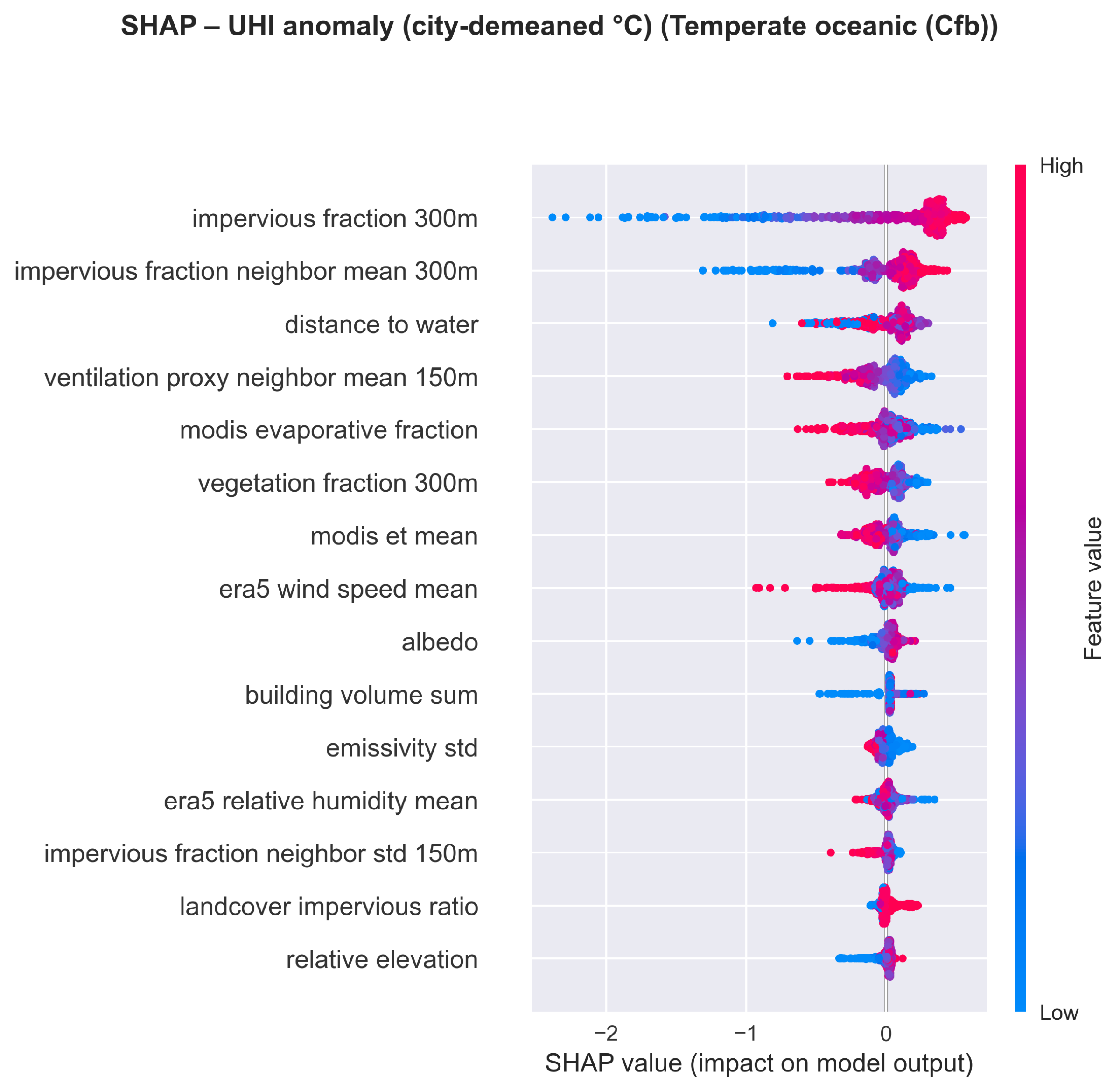
Geographic contingency isn’t noise.
It’s the signal.

Schwaab et al. (2021) Nat. Comms. · Giannopoulou et al. (2011) Athens basin. · Stewart & Oke (2012) LCZ.

[7:05 — 40s. Pause deliberately before "the signal."] Same model, same features — but the SHAP hierarchy shifts by climate. Mediterranean: albedo and built-up index dominate. Temperate: impervious fraction. Each city needs its own strategy. One-size-fits-all guidance fails. This is AI Localism in practice — the model calibrates itself to local context. Geographic contingency isn't noise. [PAUSE] It's the signal. [Q&A: Athens elevation SHAP = 0.12 — basin creates katabatic flows and thermal inversions. Vegetation importance varies 3× between Mediterranean (moisture-constrained) and temperate (evapotranspiration effective). Different feature interaction structures, not just an intercept shift. EU "increase urban greening" guidance ignores this.]

WhyHowFindingsAction

Regression→Classification→Scenarios

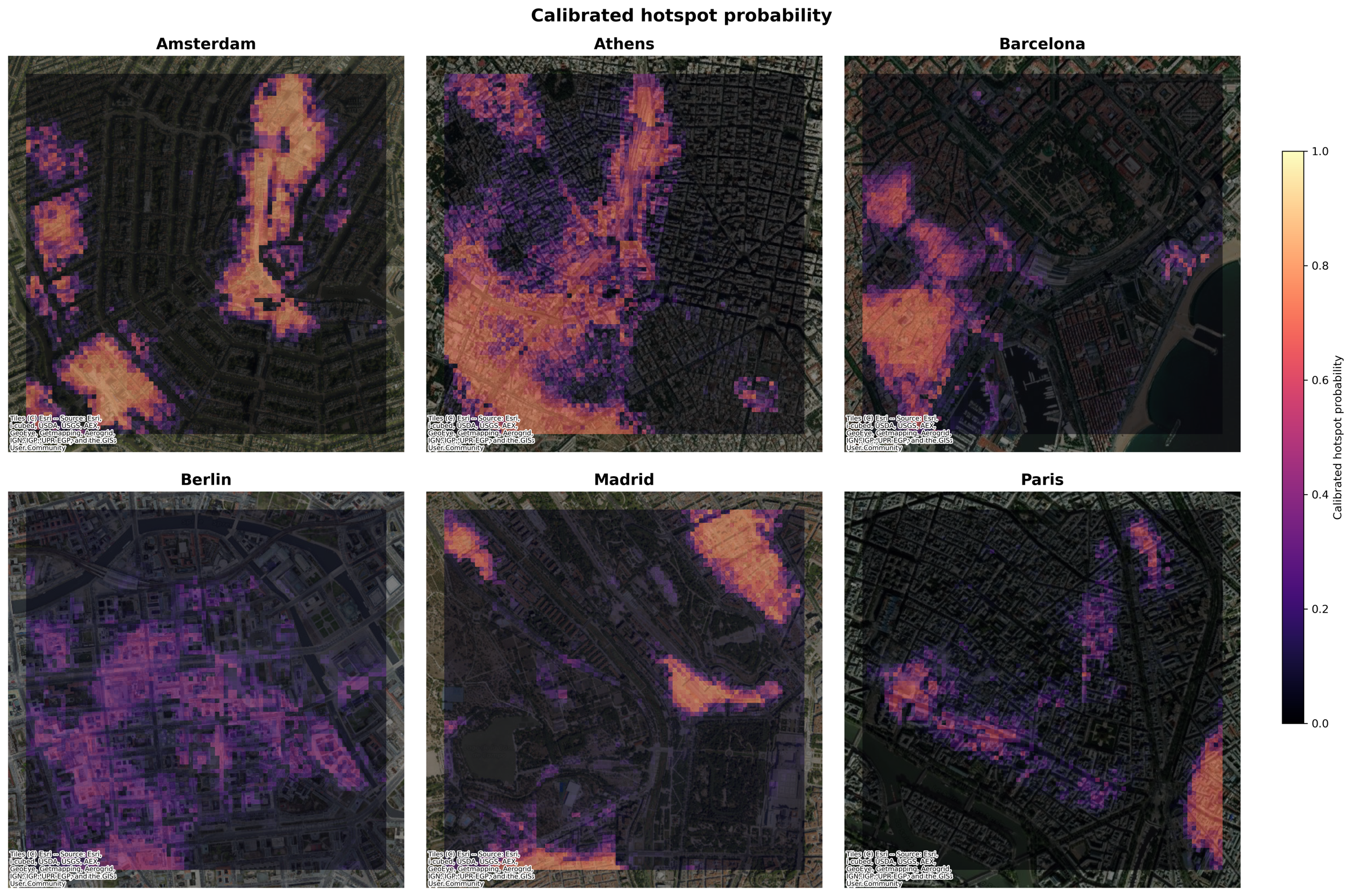
From Temperature to Risk: Classifying Hotspots

The regression tells us how hot each cell is. But planners need to know which areas are dangerously hot. That’s a classification problem: we turn continuous temperature into a binary risk flag.

XGBoost classification, upweighted to catch rare hotspots
Calibrated probabilities: when the model says 0.7, it means 70%
Threshold set to catch at least 60% of real hotspots

AUC 0.911

6,389 of 40,344 cells (15.8%) classified as hotspots
Athens: 30.8% vs Paris: 7.2%

Calibrated hotspot probability surfaces across six cities

Chen & Guestrin (2016) XGBoost. · Platt, J. (1999) Probabilistic outputs for SVMs. · Santamouris, M. (2020) Heat vulnerability.

WhyHowFindingsAction

Regression→Classification→Scenarios

Where Heat Meets Vulnerability

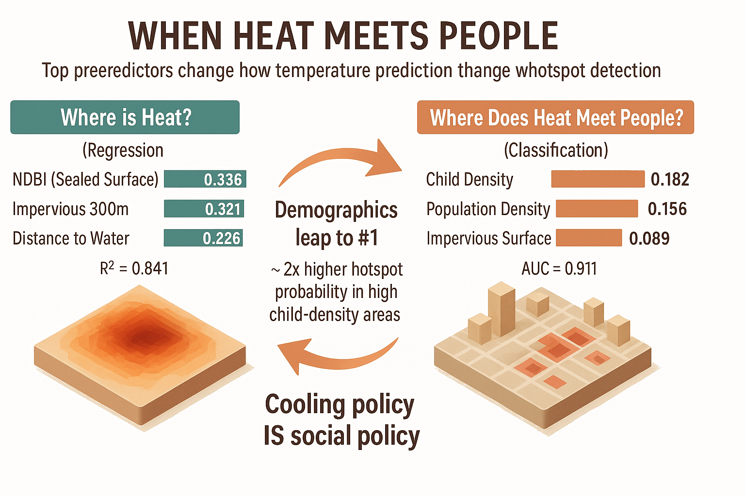
Temperature prediction to hotspot classification: demographics leap to #1

When classifying hotspots, child density becomes #1. ~2× higher hotspot probability in vulnerable areas.

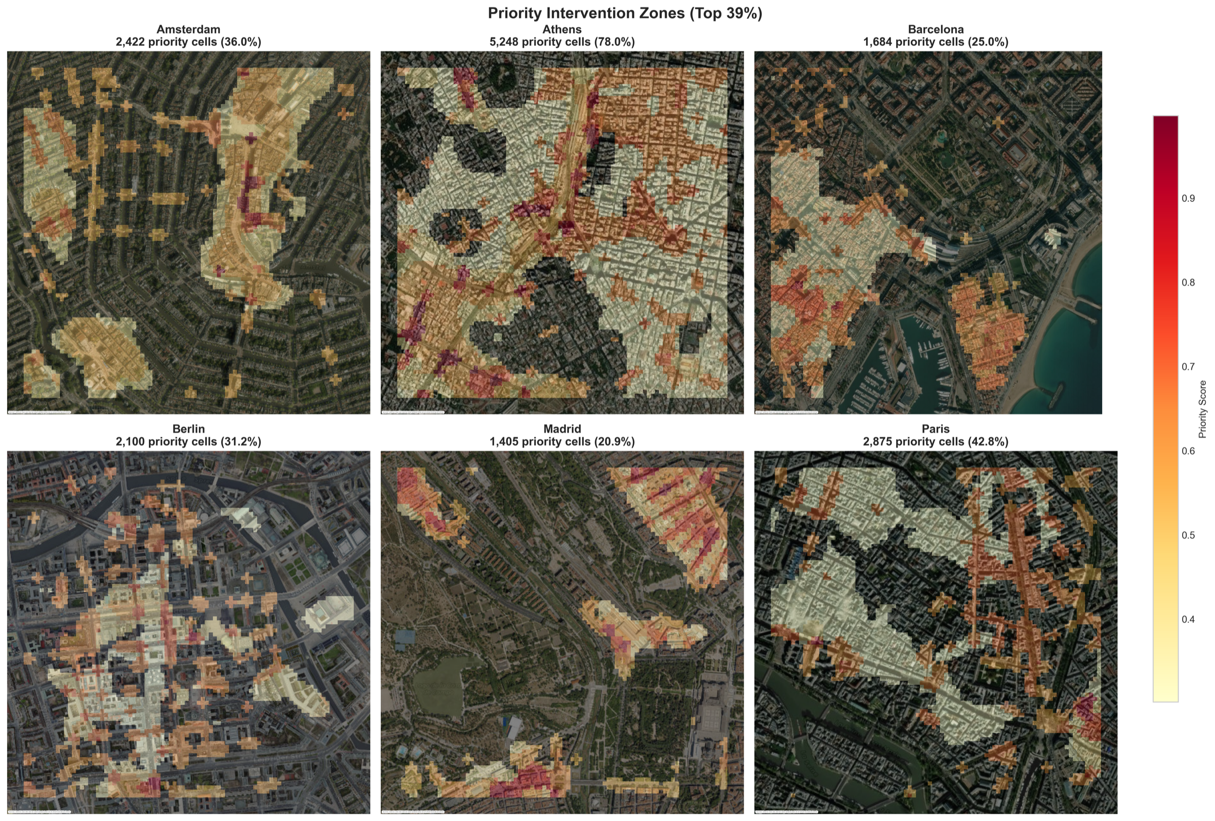
Priority intervention zones across six cities

Priority: Heat risk (40%) + Vulnerability (35%) + Cooling potential (25%)

Santamouris (2020) Heat vulnerability. · Kovats & Hajat (2008) Annu. Rev. Public Health. · Hoffman et al. (2020) Heat inequality.

WhyHowFindingsAction

Regression→Classification→Scenarios

How We Test Interventions

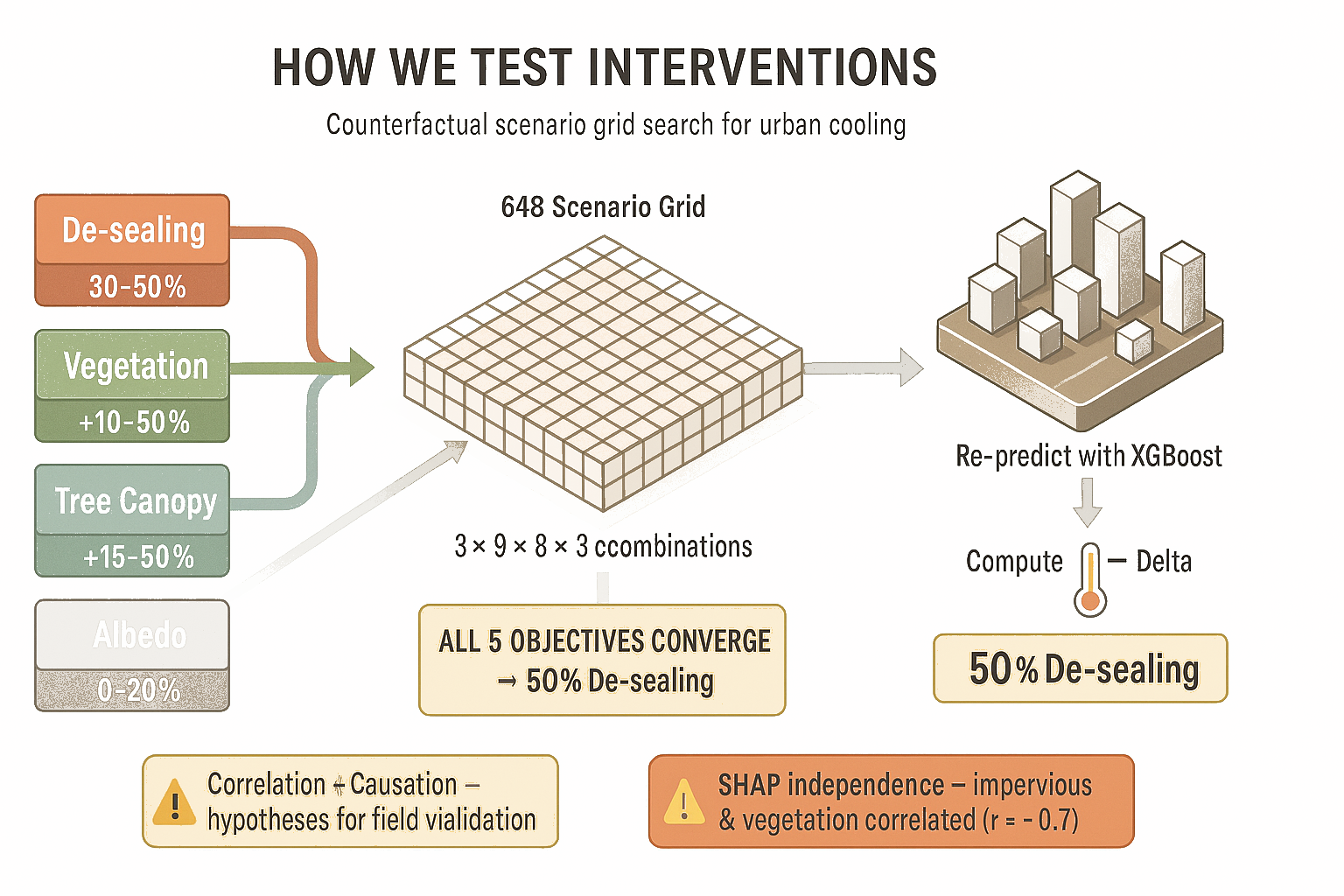
Counterfactual scenario grid search: 4 levers × 648 combinations → re-predict → convergence on 50% de-sealing

Process per scenario

Modify features in priority zones (top 10%)
Re-predict with blend model
Compute cooling Δ vs. baseline
Rank by cooling and cost-effectiveness

⚠ Limitations

Correlation ≠ causation: predictions are hypotheses for field validation

Feature correlation: impervious & vegetation (r≈−0.7) partially double-count cooling

All 5 objectives converge → 50% de-sealing

Counterfactual grid: itertools.product over 4 levers, bootstrapped 500×. Priority zones: 40% heat + 35% vulnerability + 25% cooling potential.

[9:00 — 40s] How do we go from diagnosis to prescription? Four levers: de-sealing, vegetation, tree canopy, albedo. 648 combinations, each bootstrapped 500 times. [POINT to limitations box] Two honest caveats. First: correlation, not causation — these are hypotheses for field validation. Second: correlated features may double-count some cooling when you de-seal and plant on the same surface. Despite this, every objective function converges on the same anchor. [Q&A: "Why max 50%?" — Physically plausible target from literature. Grid can't discover beyond bounds. "Bootstrap 500×?" — CIs ±0.04°C reflect model uncertainty, not real-world. "Why top 10%?" — Focus resources where heat, vulnerability, and cooling potential intersect. Weights 40/35/25 stable across ±10%.]

WhyHowFindingsAction

Regression→Classification→Scenarios

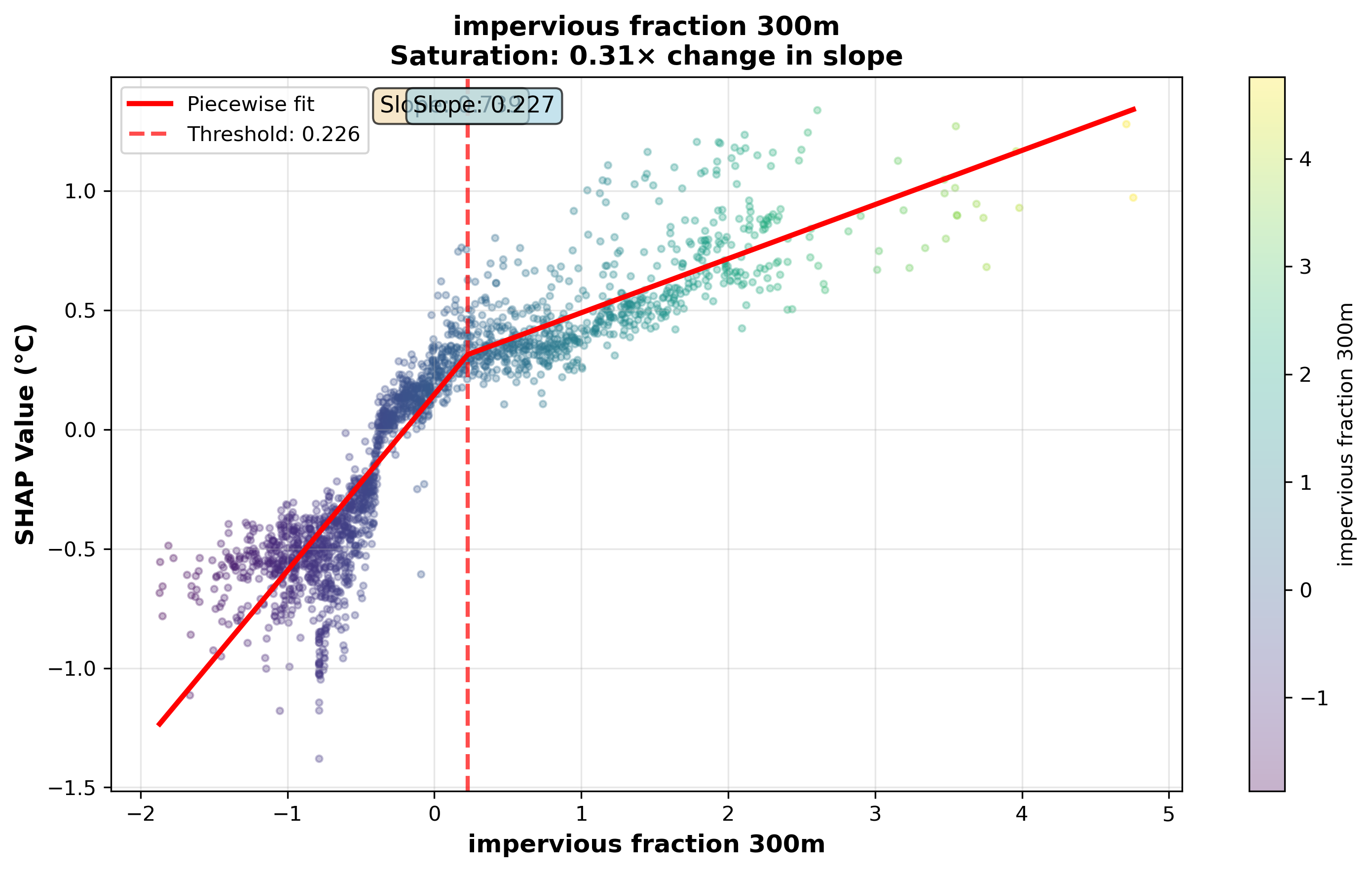
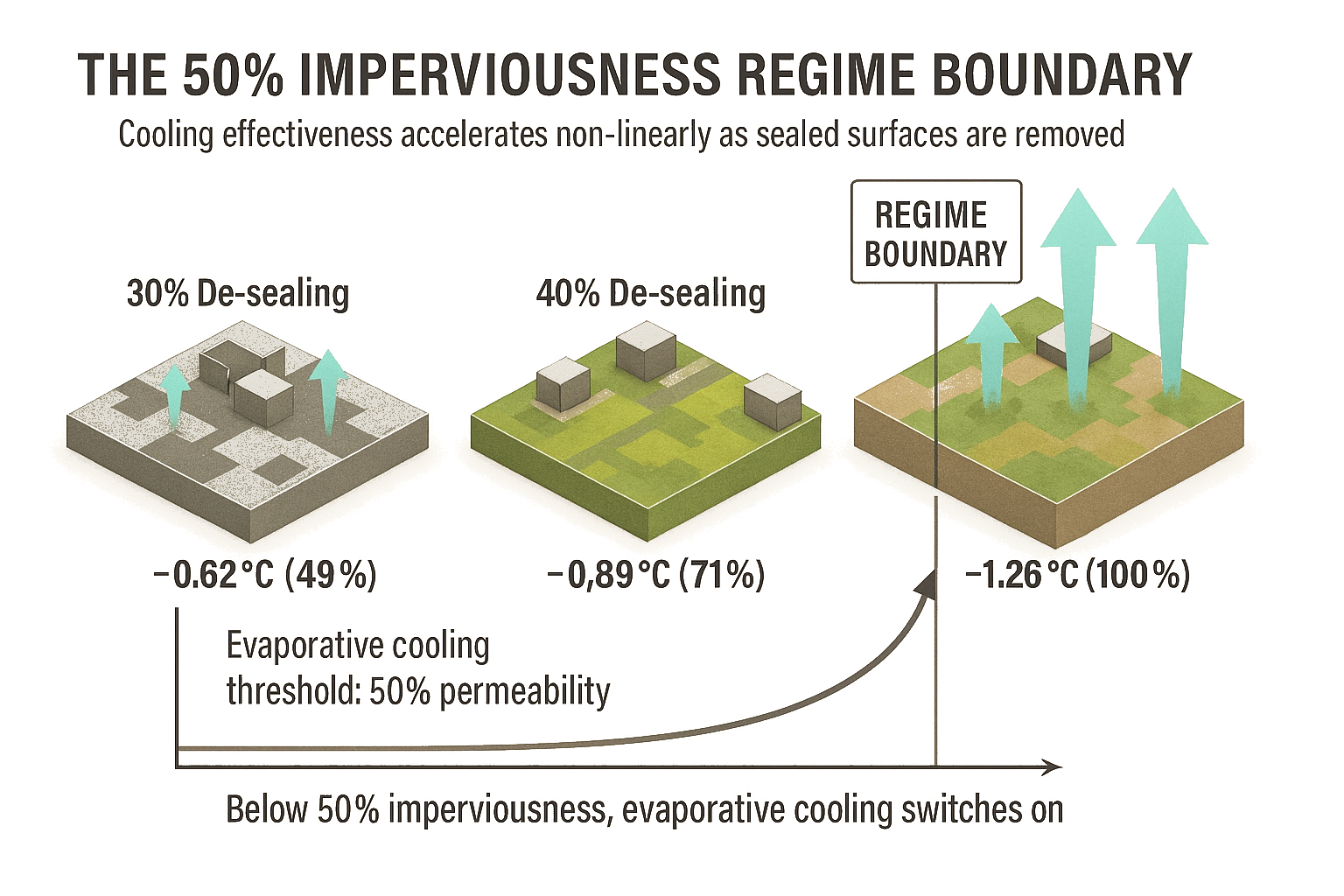
The 50% Regime Boundary

We know where hotspots are and what drives heat. Now the prescription question: how much change is enough? We tested four levers in a full grid search: depaving (30-50%) · vegetation (+10-50%) · tree canopy (+15-50%) · albedo (+0-20%) = 648 combinations, each bootstrapped 500 times.

All optimal strategies converge on 50% de-sealing. Below this threshold, evaporative cooling pathways become viable — a threshold effect.

Strategy	Depaving	Vegetation	Trees	Albedo	Cooling
Maximum	50%	+50%	+50%	+20%	−1.27°C
Cost-effective	50%	+10%	+20%	0%	−1.20°C

95% of maximum cooling with substantially fewer resources.

$SHAP dependence plot showing impervious fraction threshold at 300m$ Regime boundary diagram illustrating the nonlinear cooling response at 50% de-sealing threshold where evaporative cooling pathways become viable

Regime boundary diagram illustrating the nonlinear cooling response at 50% de-sealing threshold where evaporative cooling pathways become viable

Oke et al. (2017) Urban Climates. · Gunawardena et al. (2017) Sci. Total Environ.

[9:40 — 50s. POLICY SLIDE — deliver clearly.] 648 combinations. Every optimal strategy converges on 50% de-sealing. The response is non-linear: 30% gets half the cooling, but 50% unlocks the full threshold where evapotranspiration becomes viable. The cost-effective strategy: 95% of maximum cooling with far fewer resources. Those confidence intervals overlap — statistically equivalent. You don't need the kitchen sink. De-seal, add modest vegetation, and you're there. [IF CHALLENGED on feasibility]: "We're not asking cities to tear up streets overnight. We're asking them to make different choices when they resurface — which happens on a 10-15 year cycle." [Q&A: Max −1.27°C (CI 1.23-1.31). Cost-effective −1.20°C (CI 1.16-1.24). CIs overlap. SHAP dependence inflection at ~50%, consistent with Oke's regime boundary. These are hypotheses for field validation, not causal claims.] [Q&A DEPAVING FEASIBILITY — see comprehensive reference in Q&A slide notes.] [CHECKPOINT: ~10:30]

WhyHowFindingsAction

Regression→Classification→Scenarios

What Should Each City Do?

Same anchor everywhere: de-seal first. Supporting levers change by climate and morphology.

Athens Csa

−1.45°C

95% sealed · 78% priority

e.g. permeable paving in basin-floor neighbourhoods like Omonia

Barcelona Csa

−1.31°C

95% sealed · 25% priority

e.g. opening sealed Eixample courtyards, Superblocks-style depaving

Paris Cfb

−1.22°C

94% sealed · 44% priority

e.g. OASIS schoolyard depaving, extending Seine corridor cooling

Berlin Cfb

−1.08°C

94% sealed · 30% priority

e.g. Schwammstadt sponge-city approach in polycentric cores

Amsterdam Cfb

−0.92°C

93% sealed · 36% priority

e.g. cool surfaces + permeable paving (canals already cap water cooling)

Madrid Csa/BSk

−0.89°C

91% sealed · 21% priority

e.g. cool roofs + drought-tolerant planting (avoid water-intensive greening)

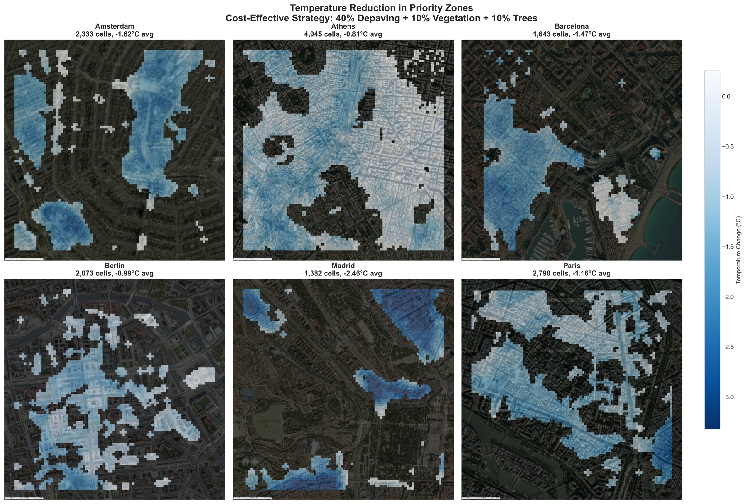
Predicted cooling from cost-effective intervention

Predicted cooling from cost-effective strategy

Gunawardena et al. (2017) Sci. Total Environ. · Giannopoulou et al. (2011) Athens basin.

[10:30 — 40s. Don't read every card — point to contrasts.] Athens gains the most — minus 1.45 degrees — because it starts worst: 95% sealed, 78% priority. Amsterdam the least, because canals already saturate water cooling. Mediterranean cities cluster at the top. Oceanic in the middle. Madrid is the outlier — semi-arid, so water-intensive greening would be counterproductive. Each card has cooling potential and priority percentage — policy makers see their headroom instantly. [Q&A: Athens 95.2% impervious, basin traps heat. Barcelona: Eixample interiors are prime targets — Bárbara Pons Giner in audience. Amsterdam: 90% cells within 200m of water. Madrid: existing canopy 21.7%, drought-tolerant species needed. "Why Athens most?" — Highest sealing + Mediterranean amplification + basin. "Why Madrid least?" — Existing canopy + semi-arid limits evaporative headroom.]

WhyHowFindingsAction

Co-Benefits & Equity Safeguards

The cost-effective strategy still includes +20% tree canopy. This isn't "stop planting trees". It's "invest in the surface beneath, not just the canopy above."

⚠ Green gentrification risk

Greening raises property values and can displace the people it aims to protect. Documented in Barcelona Superblocks and NYC’s High Line.

Our vulnerability weighting (35%) targets current vulnerable populations, but the model can’t prevent market dynamics. That requires policy.

The model says where. Communities decide how.

Gunawardena et al. (2017) Sci. Total Environ. · Anguelovski et al. (2019) Green gentrification. · Hoffman et al. (2020) Heat inequality. · Eyni et al. (2025) Scientific Reports.

[11:10 — 35s] De-sealing delivers four wins: cooler streets, fewer floods, more biodiversity, groundwater recharge. One surface intervention, four outcomes. But — [POINT to warning box] cooling investments without anti-displacement policies risk improving places while displacing people. The model says where. Communities decide how. This is responsible AI by design — governance embedded, not bolted on. [AUDIENCE: If Daniela Rizzi raises NbS: "De-sealing creates the soil conditions that make NbS viable. You can't plant into sealed ground. We're building the foundation for your NbS programme."] [Q&A: Anguelovski 2019: greening → property values → displacement. Barcelona Superblocks and NYC High Line documented this. Policy: rent stabilisation, community land trusts, participatory budgeting.]

WhyHowFindingsAction

Three Insights for Urban Heat Policy

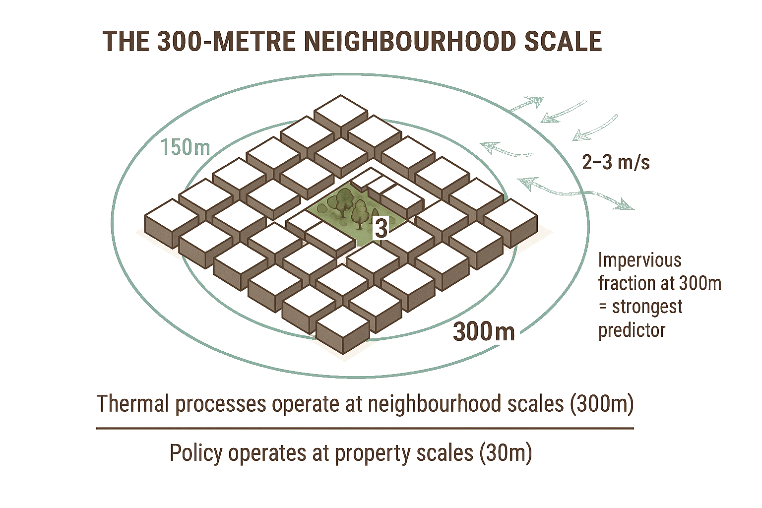
Heat is a neighbourhood problem

Cooling propagates 300 m under wind. Coordinated action across blocks, not plots.

Surface matters more than canopy

Permeability drives 3× more cooling than vegetation. De-sealing deserves equal investment.

Every city needs its own strategy

Same tree cools 8–12°C in Berlin but 0–4°C in Athens. Geography is the signal.

Oke et al. (2017) 300m advective transport. · Schwaab et al. (2021) Nat. Comms. · Eyni et al. (2025) Diversified depaving reduces health disparities more than tree-only.

WhyHowFindingsAction

What This Framework Cannot Do

Daytime only: Landsat passes at 10:30 AM, not nighttime when mortality peaks
Correlations, not causes: the 50% threshold needs field validation before policy
30m resolution: screens neighbourhoods, not individual streets
Uneven coverage: street-level imagery covers 29–71% by city

But: GEE features hold the top 8 SHAP positions — satellite data alone carries most of the signal. Any city with free Landsat access can run this pipeline tomorrow.

Waiting for perfect evidence while heatwaves kill thousands is itself a policy choice.

Oke et al. (2017) Diurnal UHI cycle, Urban Climates. · Cheval et al. (2024) Research gaps, Climate Risk Management. · Voogt & Oke (2003) Thermal remote sensing.

Every city can start
shaping cooler cities
today.

Open data. Open tools. Open method.
61,000 deaths demand tools that work now, with data cities already have.

References

Anguelovski, I. et al. (2019) Green gentrification. Landscape Urban Plan.

Ballester, J. et al. (2023) Heat-related mortality in Europe, summer 2022. Nature Medicine, 29(7), 1857–1866.

Ballester, J. et al. (2025) Heat-related mortality in Europe, summer 2024. Nature Medicine.

Camps-Valls, G. et al. (2025) AI for modeling and understanding extreme weather and climate events. Nature Communications, 16, 1919.

Chen, T. & Guestrin, C. (2016) XGBoost. Proc. ACM SIGKDD, 785–794.

Cheval, S. et al. (2024) Systematic review of UHI. Climate Risk Mgmt., 44.

Eyni, A. et al. (2025) Distributional outcomes of UHI reduction pathways. Scientific Reports, 15, 93896.

Fujiwara, K. et al. (2026) VoxCity: 3D city model generation. Comput. Environ. Urban Syst.

Giannopoulou, K. et al. (2011) Athens urban heat island. Climatic Change, 104(3).

Gorelick, N. et al. (2017) Google Earth Engine. Remote Sens. Environ., 202, 18–27.

Gunawardena, K. et al. (2017) Evaporative cooling in urban areas. Sci. Total Environ., 590, 758–775.

Hoffman, J. S. et al. (2020) Historical housing policies and intra-urban heat. Climate, 8(1), 12.

Hou, Y. et al. (2024) GlobalStreetscapes. ISPRS J. Photogramm.

Kovats, R.S. & Hajat, S. (2008) Heat stress and public health. Annu. Rev. Public Health, 29.

Lundberg, S. & Lee, S. (2017) SHAP values. NeurIPS, 30.

Milojevic-Dupont, N. et al. (2023) EUBUCCO. Scientific Data, 10, 146.

Oke, T.R. et al. (2017) Urban Climates. Cambridge University Press.

Santamouris, M. (2020) Heat vulnerability. Energy and Buildings.

Schwaab, J. et al. (2021) Urban trees reducing LST in European cities. Nat. Comms., 12, 6763.

Seneviratne, S.I. et al. (2021) Extreme events in a changing climate. IPCC AR6 WG1, Ch. 11.

Stewart, I.D. & Oke, T.R. (2012) Local Climate Zones. BAMS, 93(12), 1879–1900.

Yap, W. et al. (2023) Urbanity: automated modelling and analysis of multidimensional networks. npj Urban Sustainability, 3, 45.

Questions?

Open data · Open tools · Open method

Code & Data

gerardo.ezequiel.22@ucl.ac.uk

Gerardo Ezequiel Martin Carreno · UCL CASA · The Bartlett

═══════════════════════════════════════════════ PROJECT SUMMARY ═══════════════════════════════════════════════ "Shaping Cool Cities" is a data-driven framework for diagnosing and prescribing urban heat interventions across six European cities (Amsterdam, Athens, Barcelona, Berlin, Madrid, Paris). It fuses 118 features from five open-source tools — Google Earth Engine, VoxCity, Urbanity, GlobalStreetscapes, EUBUCCO — into a three-stage pipeline: (1) XGBoost regression predicts UHI anomalies (blended R² = 0.841), (2) classification identifies hotspots (AUC = 0.911) weighted by vulnerability, (3) counterfactual scenario grid search tests 648 intervention combinations. Key finding: surface permeability (de-sealing) drives 3× more cooling than vegetation alone. All optimal strategies converge on 50% de-sealing as the anchor intervention. The cost-effective strategy achieves 95% of maximum cooling. Geographic contingency — not noise — is the signal: the same intervention works differently in Mediterranean vs temperate climates. ═══════════════════════════════════════════════ KEY NUMBERS AT A GLANCE ═══════════════════════════════════════════════ • 40,344 grid cells, 30m resolution, 6 cities • 118 features from 5 open-source tools • Global R² = 0.695, Blended R² = 0.841 • Error reduction: 48% (unexplained variance 0.305 → 0.159) • City R²: Paris 0.932, Barcelona 0.926, Amsterdam 0.880, Athens 0.730, Berlin 0.727, Madrid 0.718 • AUC = 0.911 (hotspot classification) • 6,389 hotspot cells (15.8% of total) • 15,734 priority zone cells (39%) • SHAP: surface permeability 21%, water 13%, vegetation 7% • 648 intervention combos, bootstrapped 500× • Max cooling: −1.27°C. Cost-effective: −1.20°C (95% of max) • Blend weights: global −0.151, Cfb +0.764, Csa +0.647 ═══════════════════════════════════════════════ COMMON QUESTIONS — PREPARED ANSWERS ═══════════════════════════════════════════════ Q: "Why XGBoost and not deep learning?" A: Three reasons. (1) SHAP TreeExplainer gives exact Shapley values; neural SHAP is approximate. (2) XGBoost matches/beats neural nets on tabular data (Grinsztajn et al. 2022). (3) 40K cells is modest for DL. Explainability over marginal accuracy. Q: "This isn't causal." A: Correct. The scenario grid generates testable hypotheses for field validation, not causal claims. XGBoost captures associations. Before-after monitoring is the next step. We're explicit about this in limitations. Q: "Why not ENVI-met or CFD?" A: CFD: one block in hours. We: 40,000 cells across 6 cities in one pipeline run. Complementary — our priority zones tell you WHERE to deploy detailed CFD. Q: "How long for a new city?" A: Under half a day with existing Landsat. GEE extraction ~2 hours, training ~30 min, scenarios ~1 hour. Bottleneck: vulnerability data curation. Q: "Is 50% de-sealing realistic?" A: Yes, it's already happening: • Barcelona Eixample Green Axes (2020-23): permeable surface 1%→15%, peak surface temp −5°C. [Note: "503 superblocks by 2030" was Colau-era; Collboni admin paused new expansions. Bárbara Pons Giner from Barcelona Regional is in the audience.] • Paris OASIS: 72 of 770 schoolyards transformed, 73 ha asphalt targeted, 2-4°C cooling. • Netherlands Tegelwippen: 14M+ tiles removed since 2020, ~127 ha depaved, near-zero public cost. • Berlin Schwammstadt: Blue-Green Alliance (March 2025), subsidies 10-100 €/m². • Vienna Building Code 2023: mandates unsealing inner courtyards. We're not asking cities to tear up streets overnight — we're asking different choices when they resurface on a 10-15 year cycle. Q: "What about costs?" A: Basic removal: 16-25 €/m². Full green replacement: 80-140 €/m². NbS documented 50% more cost-effective than grey alternatives (Interreg Europe). Q: "Underground utilities?" A: Main barrier in historic cores. Heritage layers limit excavation to 30-50 cm. Strategy: target post-war areas, schoolyards, parking lots first — shallow asphalt, simple soil, minimal utilities. Q: "Why does Athens gain most but have lowest R²?" A: Highest baseline imperviousness (95.2%) means maximum de-sealing headroom. Lowest R² because basin topography (katabatic flows, thermal inversions) creates dynamics the model captures imperfectly. The blend actually hurts Athens (−2.8%) because topography overrides climate-zone correction. Q: "What about nighttime?" A: Landsat overpass at 10:30 local solar time. Neighbourhood rankings preserved at night (r > 0.7). ECOSTRESS could complement. Framework sensor-agnostic — swap the LST layer. Q: "Did you include wind?" A: Indirectly: (1) 300m spatial lags (Oke's advective transport scale), (2) street betweenness centrality as ventilation proxy, (3) SVF for canyon ventilation. Direct wind integration is a next step. Q: "Why 30m and not finer?" A: MAUP tested at 30/60/90m. 60m loses 17% explained variance. 30m aligns with Landsat native resolution and radiative physics. Finer resolution would require different sensors. Q: "What about the 3× claim? Isn't it 2.4×?" A: Top-2 features per category: 3:1. Full categories: 2.4:1. Either way, surface permeability is the dominant lever. Q: "Green gentrification?" A: Real risk. Anguelovski et al. 2019 documented displacement from Barcelona Superblocks and NYC High Line. Vulnerability weighting (35%) targets current populations but can't prevent market dynamics. Requires policy: rent stabilisation, community land trusts, participatory budgeting. The model says where; communities decide how. Q: "How does this connect to UrbanAI?" A: Three bridges. (1) AI Localism: the hierarchical blend calibrates to local context — geographic contingency is the signal. (2) Augmented intelligence: SHAP gives planners the "receipt" for every prediction — AI as co-pilot. (3) Responsible AI: vulnerability weighting, open data, open tools, governance embedded not bolted on. ═══════════════════════════════════════════════ POLICY CONTEXT ═══════════════════════════════════════════════ • EU Nature Restoration Law (Aug 2024): no net loss of urban green by Dec 2030, increasing trend from Jan 2031. National plans due July 2026. • EU Soil Strategy 2030: "no net land take by 2050" • REGREEN project: European depaving guidelines (Zenodo, 2022) • Heat = among the deadliest natural hazards in Europe. 2003: ~70K deaths. 2022: 61,672. 2024: 47,690. ═══════════════════════════════════════════════ NARRATIVE TIMING SUMMARY (15 min) ═══════════════════════════════════════════════ ACT 1 — WHY (0:00–1:55) Slide 1 Title [0:00 — 15s] Slide 2 Hook [0:15 — 30s] Slide 3 Three Gaps [0:45 — 40s] Slide 4 Study Areas [1:25 — 30s] ACT 2 — HOW (1:55–6:15) Slide 5 Data Sources [1:55 — 20s] Slide 6 GEE [2:15 — 25s] Slide 7a Urbanity [2:40 — 20s] Slide 7b Streetscapes [3:00 — 15s] Slide 7c EUBUCCO [3:15 — 15s] Slide 8 VoxCity [3:30 — 30s] Slide 9 Pipeline [4:00 — 30s] Slide 10 XGBoost [4:30 — 40s] Slide 11 Validation [5:10 — 35s] Slide 12 Performance [5:45 — 30s] ACT 3 — FINDINGS (6:15–10:30) Slide 13 SHAP [6:15 — 50s] ★ central finding Slide 14 Geography [7:05 — 40s] ★ AI Localism Slide 15 Hotspots [7:45 — 35s] Slide 16 Vulnerability [8:20 — 40s] ★ equity pivot Slide 16b Interventions [9:00 — 40s] Slide 17 50% Threshold [9:40 — 50s] ★ policy anchor ACT 4 — ACTION (10:30–13:15) Slide 18 City Cards [10:30 — 40s] Slide 19 Co-Benefits [11:10 — 35s] Slide 20 Takeaways [11:45 — 40s] ★ audience memory Slide 21 Limitations [12:25 — 35s] Slide 22 Closing [13:00 — 15s] Buffer: ~1:45 for natural pauses, clicks, audience reactions.

ShapingCool Cities

Three Gaps Preventing Action

Integration

Transferability

Action

Six Cities, Three Climates

Five Data Sources, One Framework

Google Earth Engine

Urbanity

GlobalStreetscapes

EUBUCCO

Six Cities in 3D

From Prediction to Prescription

XGBoost Regression: Why This Approach?

Can We Trust the Numbers?

Does It Work Across Contexts?

What Actually Drives Urban Heat?

Geography Changes Everything

From Temperature to Risk: Classifying Hotspots

Where Heat Meets Vulnerability

How We Test Interventions

The 50% Regime Boundary

What Should Each City Do?

Co-Benefits & Equity Safeguards

Three Insights for Urban Heat Policy

Heat is a neighbourhood problem

Surface matters more than canopy

Every city needs its own strategy

What This Framework Cannot Do

References

Questions?

Shaping
Cool Cities